Introduction
Magnetic resonance imaging (MRI) employs the nuclear magnetic resonance (NMR) principle to obtain diagnostic information about biological tissues. Every nuclei with non-zero spin can be used for MRI; however, because of its natural abundance and high sensitivity to external magnetic fields, hydrogen is the most widely used. All the factors listed above amount to a high signal-to-noise ratio in hydrogen MRI (1H-MRI). Superior tissue contrast is the reason why 1H-MRI is used so extensively for soft-tissue imaging. Its ability to present anatomy is superb; however, some diseases have no anatomic findings visible or their presence is very late. Because most of the hydrogen signal comes from either fat or water, there is limit-ed biochemical information that can be obtained with standard 1H-MRI. There are techniques that extend 1H-MRI capabilities in that regard, but these are also limited. There are some other nuclei with non-zero spin that can provide a window into crucial biochemical processes. They require additional hardware and often software. For example, phosphorus magnetic resonance spectroscopy (31P-MRS) can provide information about tissue energy metabolism, phospholipids metabolism, and pH levels [1-3]. Carbon MRI (13C-MRI) can be used in metabolic imaging [4]. Helium (3He) and xenon (129Xe) can provide useful information about the lungs, which are normally outside the scope of MRI [5]. A drawback of all non-proton-based MRI techniques is a lower signal-to-noise ratio (SNR). In the case of sodium imaging, there is approximately 20,000 times less signal than in the case of 1H-MRI. This is due to lower in vivo concentration than in the case of protons, and a lower gyromagnetic ratio.
Performing sodium (23Na) MRI, tissue sodium concentration (TSC) maps can be obtained. These maps carry a plethora of useful clinical information on various tissues. A major role of sodium ions in the human body is managing membrane transport using an ionic pump and as a counter ion for balancing charges of tissue anionic macromolecules. As such, it provides information in various diseases that impact function of sodium-potassium ion pump or disrupt ion homeostasis.
It has been shown that 23Na-MRI has its place in stroke management [6], as a marker of viable tissue (only after the acute stroke phase) prior to strokectomy performed in some cases due to brain swelling. When it comes to brain tumours, 1H-MRI offers a number of useful modalities that provide indirect information about tumour characteristics. However, during radiation and chemotherapy the most important issue is the response to treatment. Here the non-quantitative nature of the 1H-MRI signal is a drawback. Several imaging techniques, like dynamic contrast enhancement (DCE), dynamic susceptibility contrast (DSC), diffusion weighted imaging (DWI), and magnetic resonance spectroscopy (MRS), expand the capabilities of proton MRI, but their limitations can impair the radiologist’s ability to correctly asses treatment response. Sodium MRI is quantitative in principle, and it has been shown that brain tumours have higher TSC than normal brain [7]. The same work points to another parameter derived from TSC and bound by some assumptions, namely cell volume fraction (CVF). Tissue sodium concentration and CVF together can evaluate extent of tumour better than conventional proton MRI [8]. It was also suggested that the prognostic potential of sodium MRI in brain tumours can be as good as isocitrate dehydrogenase (IDH) [9]. Sodium MRI has possible applications in various regions and pathologies. There are some reports of its usefulness in Alzheimer disease [10,11], kidney imaging [12], muscle pathology imaging [13], as well as body and spine imaging [14,15]. In this work, gradient echo (GRE) sequence was applied to acquire a signal used to reconstruct the TSC brain maps of healthy volunteers.
Material and methods
Magnetic resonance imaging (23Na-MRI and 1H-MRI) was performed on 37 volunteers between October 2017 and October 2018. The examined group consisted of 22 females and 15 males. The mean age of the combined group of men and women was 37 years (range 22-64 years). Twenty-nine out of the 37 studies were of acceptable quality and were processed. The remaining 8 of the 37 studies (22%) were rejected due to incomplete acquisition or artefacts caused by the patient’s movement during the study.
All volunteers had an examination performed on a MAGNETOM Prisma 3T scanner (Siemens Healthcare, Erlangen Germany) with a double tuned 23Na/1H coil (RAPID Biomedical, Rimpar Germany), which allowed both proton and sodium imaging without moving the patient.
Sodium imaging (23Na)
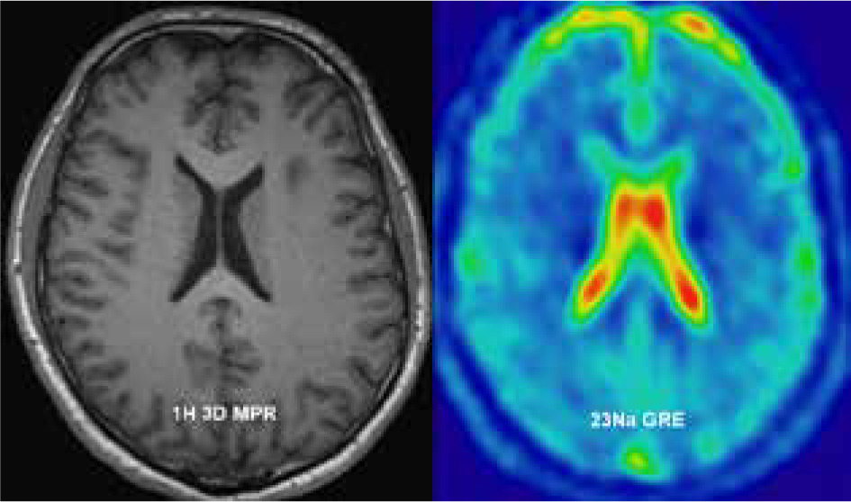
Gradient echo acquisition with radial readout scheme was performed with 4.7 mm isotropic resolution; field of view (FOV) – 300 × 300 mm, matrix (MTX) – 64; receiver bandwidth – 260 Hz/pixel; repetition time (TR) and echo time (TE) were, respectively, 100 and 2.87 ms with flip angle (FA) 90 degrees. A total of 16 slices were acquired. To achieve an acceptable signal-to-noise ratio (SNR) the acquisition was averaged (NA) 23 times, which resulted in 20 minutes of total acquisition time (Figure 1).
Proton imaging (1H)
Additionally, to assess the anatomy and for segmentation purposes, high-resolution T1 MPRage sequence was performed with 0.9 mm isotropic voxel.
Post-processing
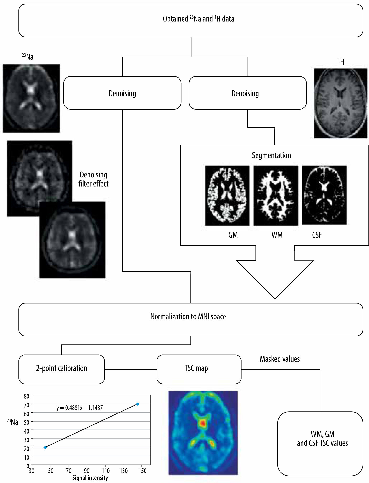
Two phantoms with known sodium concentration were positioned inside the coil for calibration. These phantoms were taped to the birdcage coil column close to the patient’s temporal bone to capture them within the FoV. Those phantoms (2 standardized 100-ml conical tubes) contained 20 and 70 mM of sodium. Using the signal intensity of these phantoms (which corresponded to known sodium concentration) a linear curve was fitted to obtain scale factors between signal intensity and sodium concentration [16]. Using these factors all acquired sodium data were recalculated into TSC using ImageJ [17] software. Then all additional steps were taken to calculate TSC values specific for tissue. The unit of all obtained values is mmol/l.
The post-processing pipeline used to acquire TSC values started with denoising of raw sodium images by means of an optimized blockwise nonlocal means denoising filter [18] to remove excess noise present in the obtained data. A similar procedure was performed on anatomic imaging. For the next step, segmentation of white matter, grey matter, and cerebrospinal fluid was performed on MPRage sequence with Statistical Parametric Mapping (SPM [19]) software. SPM uses a segmentation process that performs tissue classification, bias correction, and image registration [20] using tissue probability maps and ICBM space template for European brains [21]. Then all the acquired images were normalised into the same space (they were stretched and translated until the anatomical structures on all images overlapped). That process enabled the use of white matter, grey matter, and CSF as masks on sodium images. Subsequently, values from all voxels inside a specific mask were gathered and processed to acquire the mean sodium concentration. This process was performed using Multi-Image Analysis GUI (Mango [22]). Mean values for white matter (WM), grey matter (GM), and cerebrospinal fluid (CSF) were obtained from all sodium images (Figure 2).
Statistical analysis
Data analysis was performed with Statistica 13 software. The statistical significance threshold was set at 0.05. To assess normal distribution the Shapiro-Wilk test was performed. A t-test was performed to compare differences between TSC of WM, GM, and CSF for the whole group. For subgroups, nonparametric tests were performed because the collected data did not follow the normal distribution. To determine if there were any differences within groups, Friedman ANOVA was performed with post-hoc test. The Kruskal-Wallis test was performed to evaluate the difference in parameter values in the groups divided by sex and age. All the box-and-whiskers plots were presented with mean values as a measure of central tendency. Standard error (SE) and 1.96*SE were presented as box and whiskers respectively. The collected data were analysed in 2 different ways to lead to conclusions. Firstly, all volunteers were divided by sex and secondly by age (more and less than 35 years). The age criterion was set to ensure roughly equal groups.
Results
Using the described method and data analysis allowed us to obtain brain TSC maps for WM, GM, and CSF. The distribution of all TSC values acquired for the whole group was deemed normal; however, when data were fragmented in both ways normal distribution criteria were not met (Figure 3). With no division into groups, statistically significant differences between all the tissues (p < 0.001) were observed (Figure 4). TSC in CSF was significantly higher compared to GM and WM (p < 0.001). TSC in WM had significantly the lowest concentration compared to the other groups (p < 0.001) (Table 1).
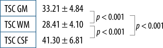
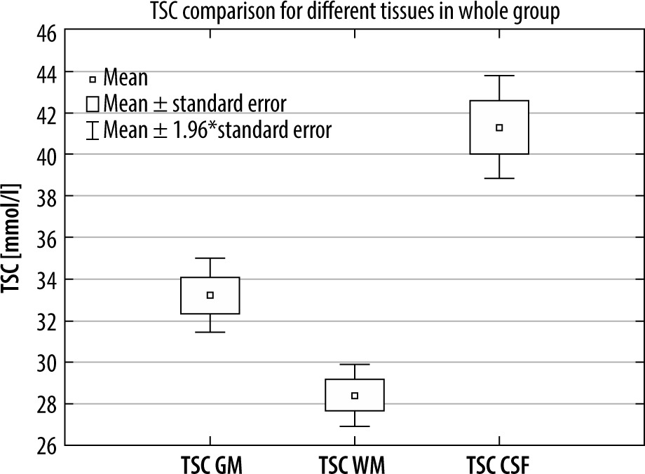
Table 1
Median TSC and quartile in men and women
| Median (quartile) | TSC GM | TSC WM | TSC CSF |
|---|---|---|---|
| Women’s brains | 33.24 (32.12-35.93) | 28.15 (26.93-31.58) | 40.11 (39.59-46.35) |
| Men’s brains | 31.09 (29.95-33.47) | 27.16 (25.32-28.47) | 39.50 (34.56-42.10) |
Volunteers were divided into groups by gender. Significant differences were found between all tissues (GM, WM, and CSF) in both groups (p < 0.001) (Figure 5). Comparing WM, GM, and CSF TSC between men and women yielded TSC WM in man vs. woman p = 0.1439, TSC GM p = 0.1212, and TSC CSF p = 1322. No significant differences in TSC were found between sexes. Although it could be observed that men tend to have lower TSC than woman in all tissues, this difference was not significant (Table 2).
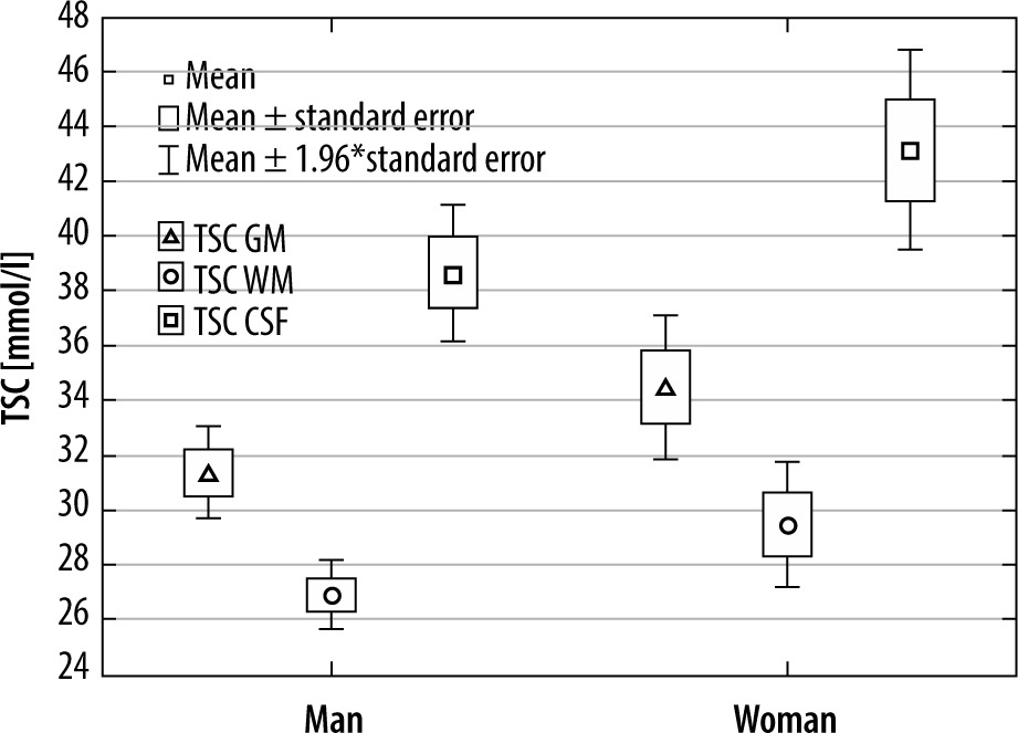
Table 2
Median TSC and quartile in younger and older volunteers
| Median (quartile) | TSC GM | TSC WM | TSC CSF |
|---|---|---|---|
| Younger than 35 | 30.12 (28.59-32.20) | 26.33 (25.15-28.12) | 38.88 (34.13-39.59) |
| Older than 35 | 34.77 (32.54-36.69) | 28.93 (27.81-32.01) | 41.50 (39.94-45.61) |
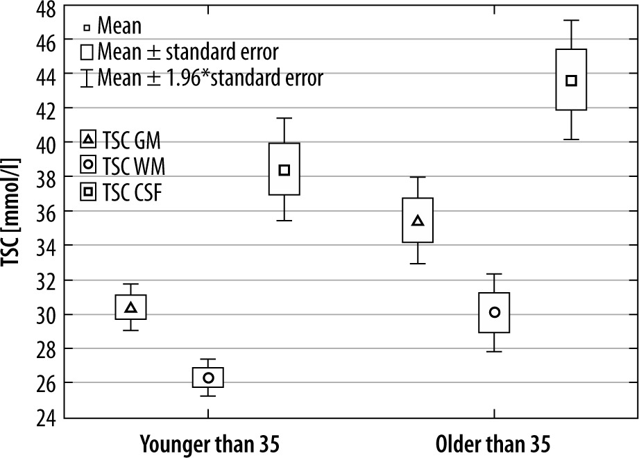
In the second approach, volunteers were divided into 2 age groups: above and below 35 years old. As in the first comparison, there was a significant difference between WM, GM, and CSF in both older and younger groups (p < 0.001 in all cases).
Comparing the TSC in the 3 considered tissue types between younger and older volunteers, TSC WM (p = 0.0085), TSC GM (p = 0.0014), and TSC CSF (p = 0.0097). In all these comparisons there was a significant difference in TSC between younger and older volunteers (Figure 6).
Discussion
Different tissue types have different TSC, which means a statistically significant difference between WM, GM, and CSF. This statement holds true in all of the subgroups despite a small number of volunteers in them. It was previously proven [6,23] that most sodium in the brain can be found in CSF and that GM has a higher concentration of sodium than WM; the results in this study are no different in that regard.
There were no differences observed between men and women in TSC in brain tissues. Although the collected data showed that men have slightly lower TSC, that difference is of no significance. According to our knowledge, no previous study analysed the differences between men and women in regards to this parameter, so no data are available for comparison. Dividing participants by age into arbitrarily chosen groups (to maintain roughly equal subgroups) yielded interesting results. As with all previous data, there were differences between TSC in CSF, WM, and GM in all subgroups. Interestingly, there were significant differences (p < 0.05) between all these parameters between younger and older participants. Younger volunteers had lower TSC in all calculated parameters. This is in contradiction to findings in another paper [24] in which the mean TSC in the whole brain was stable in all ages in healthy volunteers. Also, some sources [25] point out that overall sodium levels in healthy individuals tend to decrease with age. A possible source of the bias might be in the volunteer group itself. The oldest participant was 64 years of age, and there were only 3 people older than 50 years, which might be a drawback in characterizing the age spread of TSC.
By using a relatively long TR (100 ms), which spanned around 3 times the native sodium relaxation time (25-40 ms), correction for T1 was not of major importance for sodium quantification [26] because negligible T1 saturation occurs in this situation. However, the TE used (2.8 ms) and no correction led to considerable bias, as shown in previous papers [27]. While using a 3D radial GRE sequence a shorter echo time was not achievable. The problem with long TE can be addressed by using one of the more sophisticated sequences developed specifically for 23Na imaging [28]. Because the brain is a homogenous environment and the birdcage coil has a uniform excitation profile, B1 correction was unnecessary. However, even in these conditions, not accounting for B1 inhomogeneity might be considered a drawback. Bearing the above in mind, the values acquired for TSC should be considered as “institutional values” and they can be compared with other values acquired in the same institution, but they might not be comparable with absolute values acquired considering all the mentioned corrections. That being said, values obtained for WM in healthy volunteers in this study are similar to those presented by Romanzetti et al. [28] using a similar sequence considering all the above corrections.