Introduction
Cervical cancer develops in the cells of the cervix and the lower part of the uterus. Most cases of cervical cancer result from high-risk, sexually transmitted human papillomaviruses (HPV). According to statistics, the second most common cause of death among women is cervical cancer [1]. In 2018, most of the cases and fatalities from cervical cancer were seen in low- and middle-income countries, where access to screening on a regular basis and early intervention detection is usually low. It is important to have regular check-ups and early identification of cervical cancer, and cytological tests, such as the Pap-smear test, are among the most effective methods of early detection [2]. Cervical Pap smears are used to detect precancerous or abnormal cells within the cervix (uterus’ opening). To determine whether abnormal cells have spread, a sample is carefully taken from the cervix and analysed [3]. Due to their lower proneness to human errors, computer-aided detection methods have gained popularity in place of manual diagnosis [4]. The algorithms analyse images to determine whether the cases are healthy or diseased based on their input. In recent years there have been many publications on the use of machine learning (ML) to detect cervical cancer early [5-7]. Generally, these algorithms are trained on a given dataset for the extraction of some characteristics for classification.
It has always been the first choice for outstanding performance over classical handcrafted feature engineering to use CNNs. Developed initially for document recognition, CNNs have been extensively applied to image, video, voice, and audio processing over the past decades to solve interdisciplinary research challenges [8,9]. There are 2 components to a traditional CNN: a feature extractor and a classifier model, both of which are learned during training. In addition to CNN, there are other issues to consider. Improved performance is usually achieved by combining additional techniques with convolutional neural networks. It has been suggested that multiple CNNs can be combined to make more informed decisions. Using weighted SVMs [10], proposed aggregating multiple CNN architectures for classifying handwritten music symbols using a trainable aggregator function. An aggregation method based on fuzzy Choquet integrals was used to recognise human actions [11]. As its performance depends on tuning, this aggregator function can be considered a tuneable aggregator.
Several researchers, such as Chakraborty et al. [12], used ensemble approaches that aggregate the outputs of CNNs using sum and product rules to eliminate the need for training or tuning. Trainable aggregator functions may benefit scenarios with several classes and when the underlying classifiers provide conflicting predictions. In such instances, these algorithms may consolidate characteristics to ensure accurate classification of a sample. Tuneable and non-parametric aggregators are quite nominal when the target or output classes are limited, and the outputs of the base classifiers are not significantly divergent [13]. Because CNNs require large datasets with labelled images (Pap smears, colposcopy, and histopathology) and substantial computational resources, transfer learning is utilised, applying pre-trained models for feature extraction [14]. Transfer learning models like AlexNet, Inception, ResNet-101, and Xception have achieved high accuracy in classifying cervical cell images [15]. Because AlexNet is prone to overfitting, ResNet requires large datasets for training and is computationally expensive. Variants of Inception and Xception have been explored for diagnosing cervical cancer. Inception is computationally efficient, uses few parameters, and has an excellent prediction accuracy with relatively small datasets [16]. Xception is more efficient than Inception, with fewer parameters, and it is highly accurate even with large datasets [17].
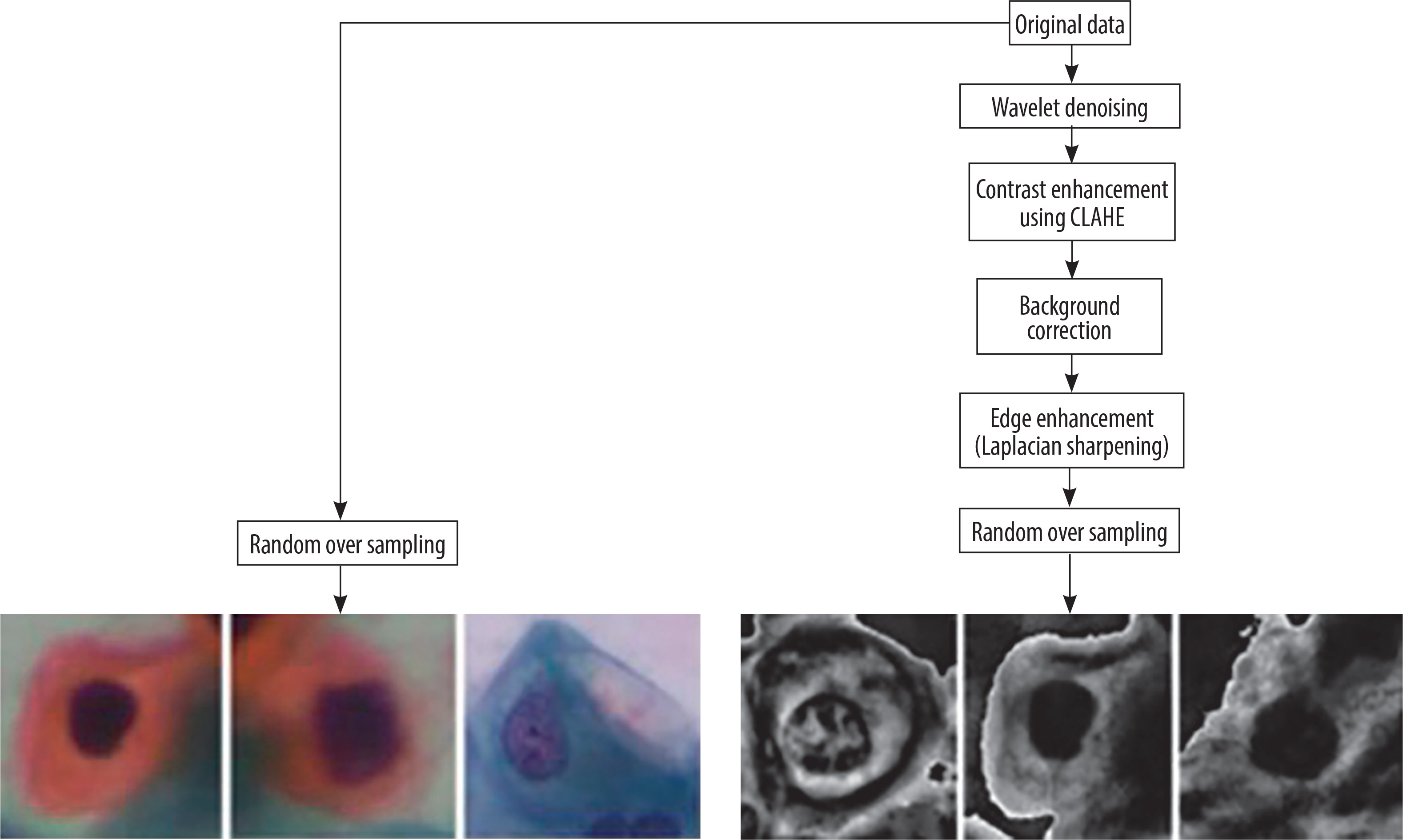
Pre-processing is required in cervical cancer diagnosis for enhancing image quality, reducing noise and improving crucial features. Pap smear images may contain noise due to uneven illumination, digitisation, or staining. Edge enhancement is required to make features like cell boundaries, nuclei, and cytoplasm distinct [18,19]. Wavelet denoising, background correction, CLAHE, and Laplacian sharpening have been used because wavelet denoising is capable of removing noise from images without blurring the edges. Background correction eliminates inconsistencies in illumination and background variations. CLAHE is used in improving image contract by utilising local histogram equalisation. Laplacian sharpening utilises a Laplacian operator to enhance edges by the detection of regions with high frequency.
By analysing the Pap-smear images, this study aimed to detect cervical cancer. The proposed method used 3 transfer learning approaches: simple CNN, Inception V3, Xception, Xception with attention, and Inception with attention. A novel ensemble method, which combines the outputs of the above models, focusing on minimising the error between observed values and ground-truth data, has been proposed. Whenever multiple predictions are available, the method will take 3 distance measures from the best possible solution for each class, i.e. Euclidean, Manhattan, and Cosine. Final predictions are calculated using de-fuzzified distance measures calculated by utilising the product rule. The authors’ main contributions of the present study are as follows:
The study proposes a new fuzzy distance-based ensemble of CNNs for classifying cervical cancer using Pap-smear images. Five CNN models and the attention mechanism are utilised for feature extraction of extra features. The model improves accuracy by minimising biases, strengthens robustness to noise, provides explainable decisions (interpretability) using fuzzy logic, and seamlessly adapts to various CNN architectures without retraining (adaptability).
There are 4 pre-processing algorithms: wavelet denoising, CLAHE, background correction, and Laplacian sharpening for edge enhancement, which are used to create the new dataset. The proposed pre-processing techniques ensure that the images in the new dataset have higher image clarity, improved segmentation, and edge and contrast enhancement, leading to more accurate classification of the cells, ultimately ensuring better diagnostic performance.
The work employs new a fuzzy distance-based aggregator function that reduces the ground-truth samples also called the ideal solution and observed samples difference. The ideal solution distances in 3 spaces are taken into account by the proposed ensemble method. The approach can effectively aggregate the base learners’ confidence scores so that the ensemble performance can be enhanced. Fuzzy logic improves the interpretability of the decision-making model by providing confidence levels for predictions instead of fixed classifications. Distance-based weighting further improves reliability by giving higher weightage to predictions that are closer to the correct class.
The model outperforms most of the state-of-the-art approaches on 2 datasets, where dataset 1 is publicly available and dataset 2 is constructed after pre-processing.
In the proposed work InceptionV3 was chosen because of its parameter savings and better performance on medium-sized datasets, where its factorised convolutions cut down on computations without sacrificing accuracy. Xception, on the other hand, substitutes regular convolutions with depth-wise separable convolutions to achieve better performance at fewer parameters for big datasets. In contrast to AlexNet, a non-deep and overfitting network, and ResNet, a computationally intensive network, both InceptionV3 and Xception strike an ideal balance between complexity and performance. Hence, they are more suitable for practical tasks such as cervical cancer classification. Existing work that uses sum or product rule-based aggregation fails where base classifiers provide contradicting outputs. Our fuzzy distance-based aggregator can better manage such conflicts, generating confidence weights based on the distance to the ideal output [15-17].
The remaining part of the work is described in various sections. Existing related research work is discussed in Section 2, while Section 3 discusses all the methods and materials utilised in developing and implementing the proposed model, such as the dataset used, techniques of pre-processing, etc. Section 4 describes the proposed model, the complete pipeline, and the main algorithmic steps used to design the model. Section 5 illustrates the results and comparisons of findings with existing work, and Section 6 presents the conclusions and future scope.
Literature review
The present section discusses approaches in existing literature on the classification of cervical cells, outlining the different methodologies proposed, their efficiency, and the challenges faced. CNNs are frequently used for cervical cell classification because they are capable of extracting hierarchical features from images of Pap smears [20]. Hemalatha et al. [21] combined fuzzy logic with CNN to classify cervical cell images. The authors claimed that the integration of interpretability of fuzzy systems with the efficiency of CNNs improved the classification accuracy. De Lima et al. [22] proposed the use of Mask R-CNN, which is capable of instant segmentation, for cervical cell classification. Ali et al. [23] proposed a hybrid model by integrating naive Bayes (NB), random forest (RF), SVM, and decision tree (DT) classifiers. The risk factor dataset of the UCI Machine Learning Repository was used for models training and testing. The study [24] explored transfer learning for classifying cervical cells, comparing 13 pre-trained deep CNN models on the relatively small and imbalanced Herlev dataset, containing Pap-smear images. The best classification accuracy of 87.02% was achieved with DenseNet-201.
The federated learning (FL) approach allows hospitals to train models independently and collaboratively improve a global model without sharing sensitive data. Nasir et al. [25] developed a federated ML model with Blockchain for data security and IoMT for data collection. Reference [26] utilised a CNN-based federated learning framework to classify cervical cell images while ensuring patient data confidentiality. The approach demonstrates high classification accuracy in both scenarios. However, limitations such as high computational demands, communication overhead in FL, and reduced accuracy in non-FL scenarios remain challenges. The study [27] explored digital twin along with CervixNet classifier for cervical cancer detection, using the relatively small SIPaKMeD dataset. Although CervixNet demonstrates high accuracy, it has dataset constraints, reducing its generalisability.
An approach was presented by Xie et al. [28] to predict the radiation dose to be administered for cervical cancer radiotherapy. For prediction, beam channel generative adversarial networks (BC-GAN) are proposed, but the dataset used is relatively small. Mathivanan et al. [29] employed deep CNN models with machine learning algorithms to detect cervical cancer using AlexNet, InceptionV3, ResNet-101, and ResNet-152. Due to its reliance on only the SIPaKMeD dataset, the study has generalisation issues. The study [20] combined Vision Transformer (ViT) with SeNet, DenseNet169, and ResNet101 models for the classification of unsegmented images of cervical cells. The authors claim that accuracy can be improved by using approaches such as cervix feature fusion (CFF) and fuzzy feature selection. The datasets used, SIPaKMeD and Mendeley, are relatively small, leading to generalisation and overfitting issues. Study [31] investigated synthetic medical images created using GANs for predicting the reappearance of cervical cancer following radiotherapy. The study aims to expand dataset diversity and availability to help overcome the limitations of real-world medical data.
Madathil et al. [32] trained a deep learning model using multiple modalities like clinical records, medical imaging, and molecular biomarkers. ConvNeXt has been used for feature extraction and CerVital Predict for predicting cervical neoplasia. The study [33] combined CNN with transfer learning for cervical cell classification. They employed pre-trained models for extracting features along with machine learning classifiers, trained using the SIPaKMeD and Herleve datasets. In 2025, Hemalatha et al. [34] proposed a self-supervised learning method in which contrastive learning is used in extracting features from unlabelled cervical cancer cell images. But self-supervised learning approaches are believed to be less accurate in comparison to supervised approaches. Another limitation of these works is the use of relatively small datasets, which may result in lack of generalisation and overfitting.
Wang et al. [35] proposed an AI-based system for detecting cervical cancer. Utilising a comprehensive real-world dataset, ResNet-18 was used for feature extraction and random forest for classification. In study [36] the authors developed the MaxViT architecture by substituting MBConv with ConvNeXtv2 blocks and replacing MLP layers with global response normalisation (GRN)-based MLPs. The study [37] combined InceptionV3 with DenseNet201 to improve cervical cell cancer prediction accuracy. The authors used pre-processing techniques like augmentation, normalisation, dataset splitting, and dimensionality optimisation for feature selection. But these studies use a relatively small database and interpretability remains a challenge.
Munshi [38] addressed the issue of class imbalance and missing data by integrating support vector machine (SVM) imputation for handling missing values, adaptive synthetic (ADASYN) sampling for class imbalance, and CNN that performs feature extraction. These are combined within a stacked hybrid ensemble model that integrates the prediction strengths of diverse ML models. The study [39] addressed the challenge of missing values by combining the K-nearest neighbours (KNN) imputer with ensemble voting classifier. Muksimova et al. [40] developed RL-CancerNet, which blends CNNs and reinforcement learning to enhance diagnosis of cervical cancer. The proposed framework was trained and evaluated on the SipaKMeD and Herlev datasets. In these works, the proposed models are evaluated on single, relatively small datasets, limiting the generalisability. Study [41] proposes a model for classifying cervical cytology images based on DenseNet121 improved with Convolutional Block Attention Module (CBAM). The combination is to improve feature representation by highlighting informative spatial and channel areas of the image, thereby attaining high classification accuracy on the SIPaKMeD dataset. But the model is limited by its dependence on a single backbone architecture with no ensemble fusion, which could limit its stability in heterogeneous clinical situations. The research [42] presents a model based on CNN with additional CBAM and parallel branches for enhanced cervical cell image feature extraction. The model was 92.82% accurate on the SIPaKMeD database with enhanced attention to diagnostically critical locations. There was no ensemble learning and external validation. No clinical deployment process was addressed.
Research gaps
According to the literature, the following are identified as the key gaps in research:
Although some works employed CNNs and pre-trained deep models (e.g. ResNet, InceptionV3, DenseNet) to classify cervical cells, applying attention mechanisms with pre-trained models to classify cervical cells has not been extensively investigated. While more recent studies [21,35] have incorporated attention mechanisms such as Squeeze-and-Excitation (SE), CBAM, and self-attention into CNNs (ResNet, DenseNet) in classifying cervical cancer, they mainly apply attention alone or with one model. This study builds upon the aforementioned research by incorporating attention-augmented CNNs into a fuzzy ensemble, thus enhancing interpretability and robustness with multiple base classifiers.
Attention mechanisms can enhance feature selection and make deep learning models more interpretable.
Single classifiers or ensemble methods such as voting classifiers and stacked ensembles are mostly utilised in research. Fuzzy distance-based aggregation is not applied to aggregate the predictions of more than a single model that might improve decision-making reliability.
The method would deliver a strong and interpretable way to obtain final classification decisions.
There have been various models (e.g. CervixNet, ViT-based models) that have been trained on relatively small sets like SIPaKMeD and Herlev, thus restraining their generalisability [27,28].
Class imbalance in cervical cancer databases is another significant issue, with the propensity to cause biased predictions in most cases. Although some research removes it by employing ADASYN or synthetic data augmentation, more efficient data augmentation methods and imbalance management strategies should be investigated [38].
Most of the current deep learning models, such as CNNs and Vision Transformers, are black boxes, and thus it becomes difficult for medical professionals to interpret the results. Fuzzy logic-based methods provide an interpretable solution but are yet to be widely hybridised with deep learning models for cervical cancer classification.
Material and methods
Dataset
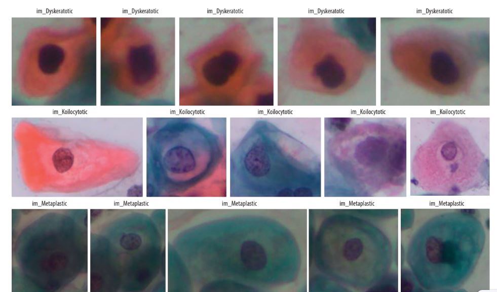
SIPaKMeD is an open-source dataset, which was used in the study. This dataset contains a total of 4049 single-cell images, which were manually retrieved from 966 cell cluster images of Pap-smear slides. Microscopic images of cells are captured with the help of a CCD camera and an optical microscope. Normal cells, abnormal cells, and benign cells fall into 5 categories: dyskeratotic, metaplastic, parabasal, koilocytotic, and superficial-intermediate (Figure 1).
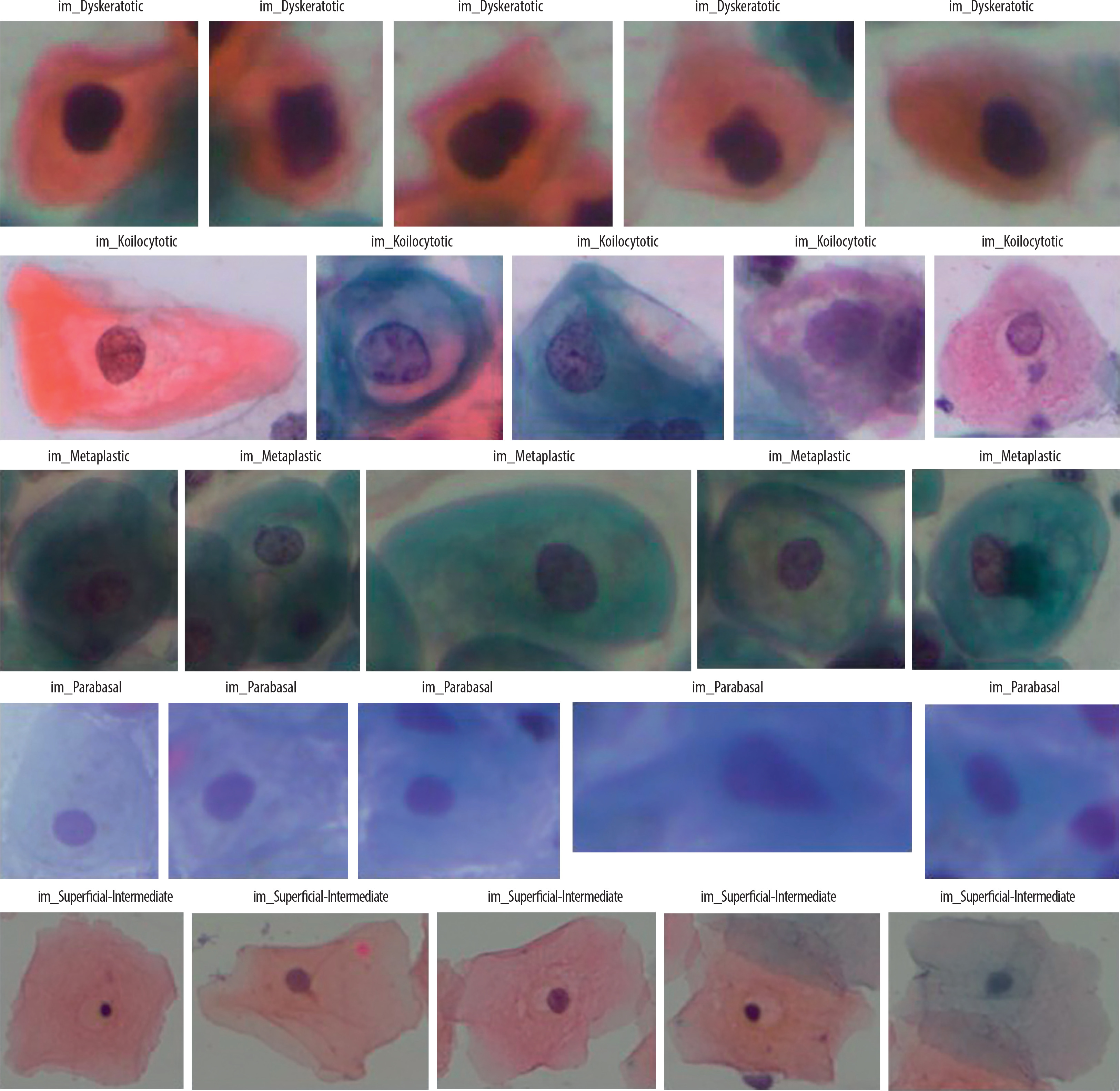
A dyskeratotic cell is a squamous cell that has undergone premature abnormal keratinisation within an individual cell or in clusters. Despite being orangeophilic, their cytoplasm is brilliant.
Koilocytic cells have vesicular nuclei similar to those of koilocytic cells. In many cases, cells with several nuclei are likely to be binucleated or multinucleated. The second category, koilocytotic cells, is mainly found in mature squamous cells, both superficial and intermediate. They appear mostly cyanophilic, very lightly stained, and characterized by a large perinuclear cavity.
Metaplastic cells are either small or large parabasal-type cells characterised by distinct cellular boundaries, sometimes exhibiting eccentric nuclei and occasionally possessing a substantial intracellular vacuole. The central staining is often light brown and contrasts with the marginal staining. The subsequent group, parabasal-cells, comprises immature squamous cells and represents the smallest type of epithelial cells seen in a standard vaginal smear. The cytoplasm is often cyanophilic and typically features a prominent vesicular nucleus.
Parabasal cells have morphological similarities to metaplastic cells, making differentiation between the 2 challenging.
The last group comprises the majority of cells obtained in a Pap test. They often present as flattened structures with round, oval, or polygonal cytoplasm, generally eosinophilic or cyanophilic. Their nucleus is centrally placed and pycnotic. Their cytoplasm is large and polygonal with well-defined boundaries, and the nuclear borders are immediately identifiable.
Pre-processing
To prepare the dataset images for better feature extraction and classification, various pre-processing techniques were utilised to improve the quality and contrast of images, and a new dataset was created.
Wavelet denoising (Haar Wavelet)
This helps to remove noise while preserving important features like edges and textures. It works by transforming the image into different frequency components and filtering out high-frequency noise [43]. The whole process done in 3 steps:
The discrete wavelet transform (DWT) is applied using the Haar wavelet, shown in Eq. 1
where LL is the approximation (low-frequency component) and LH,HL,HH are components of high frequency, containing noise.
Contrast enhancement using CLAHE
This step is used to improvise the visibility of structures in an image using a contrast limited adaptive histogram (CLAHE) [44]. The contrast is enhanced by adjusting pixel intensities in small regions while preventing over-amplification of noise using the following steps:
The image is divided into N×N tiles, N = 8.
A histogram is computed for each tile and clipped at a threshold T to avoid excessive contrast amplification.
The histogram is redistributed, and new pixel intensities are computed using Eq. 4.
where Hclip is the excess part of the histogram after clipping.
Background correction
This step removes uneven lighting effects and enhances the cell structures. Uneven illumination in images was corrected by estimating the background and subtracting it from the original image using Eq-6. For morphological opening, Eq-5 (erosion followed by dilation) was used to extract the background.
where B(x, y) is the estimated background, K is the structuring element called kernel
Edge enhancement (Laplacian sharpening)
This step was used to sharpens the image by highlighting intensity transitions (edges). The Laplacian operator detects edges and is eliminated from the image to enhance contrast. The Laplacian filter is applied using Eq-7.
where
The enhanced image was obtained by subtracting the fraction α of the Laplacian from the original image, represented in Eq-8.
where α controls the sharpening strengths.
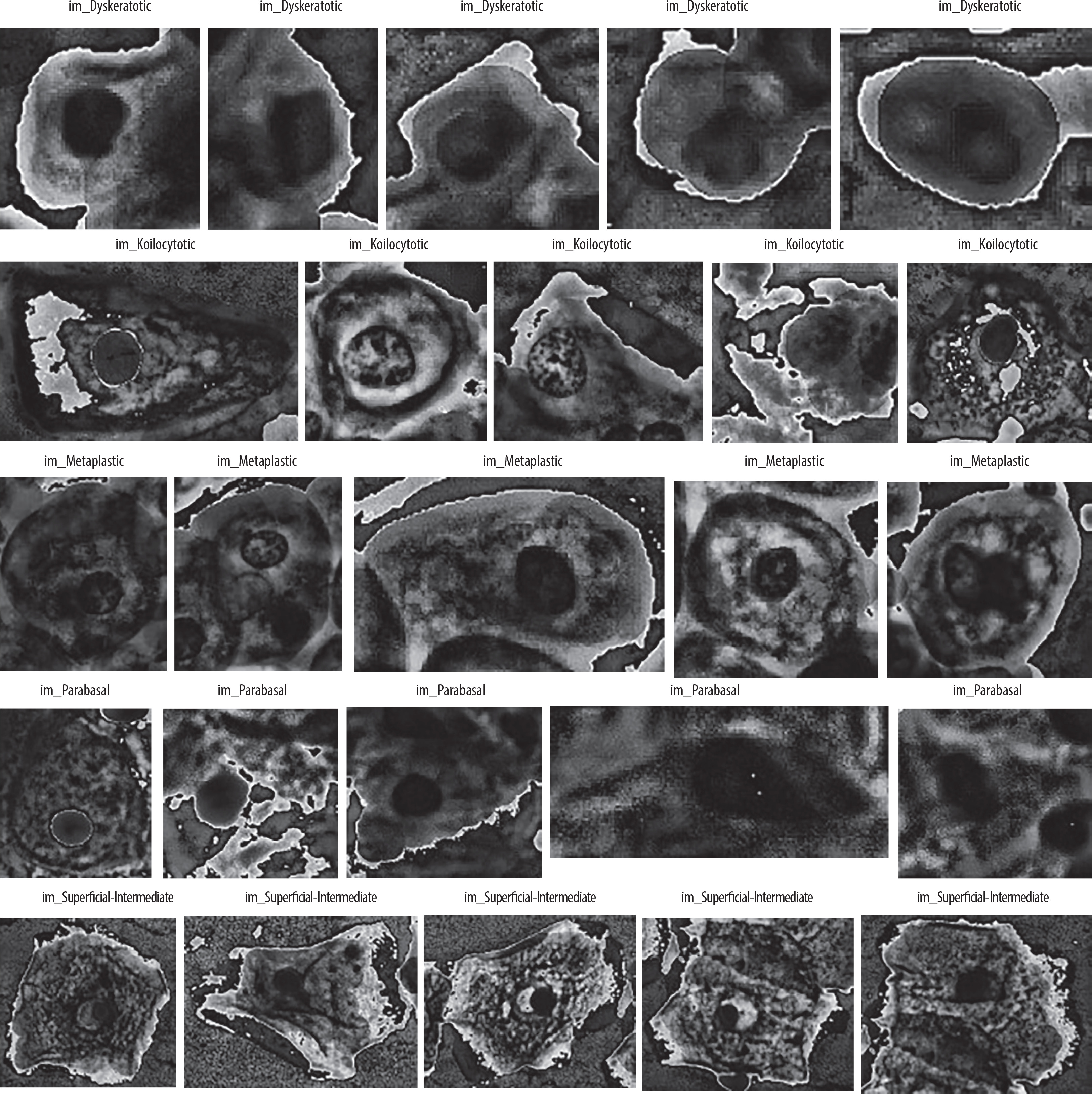
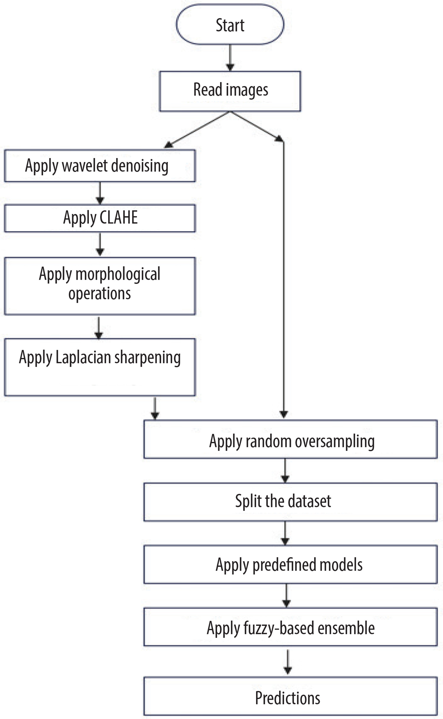
Figure 2 shows the flow diagram of creation of new dataset, and Figure 3 shows the sample images from the new dataset achieved after all steps of pre-processing.
Random oversampling
Random oversampling (ROS) is a data balancing method that is used in balancing the dataset if it is imbalanced as per defined categories. It expands the dataset by augmenting the minority class samples through random duplication of existing samples, without generating new data. This helps equalise the class distribution, letting the classifier learn patterns from both the classes more effectively.
Algorithm-1 shows the important steps used in the random oversampling. Let X is the feature set, y is the label set, Cmaj represents majority class, Cmin represents minority class, and Nmaj and Nmin are samples of majority and minority classes, respectively.
Proposed framework
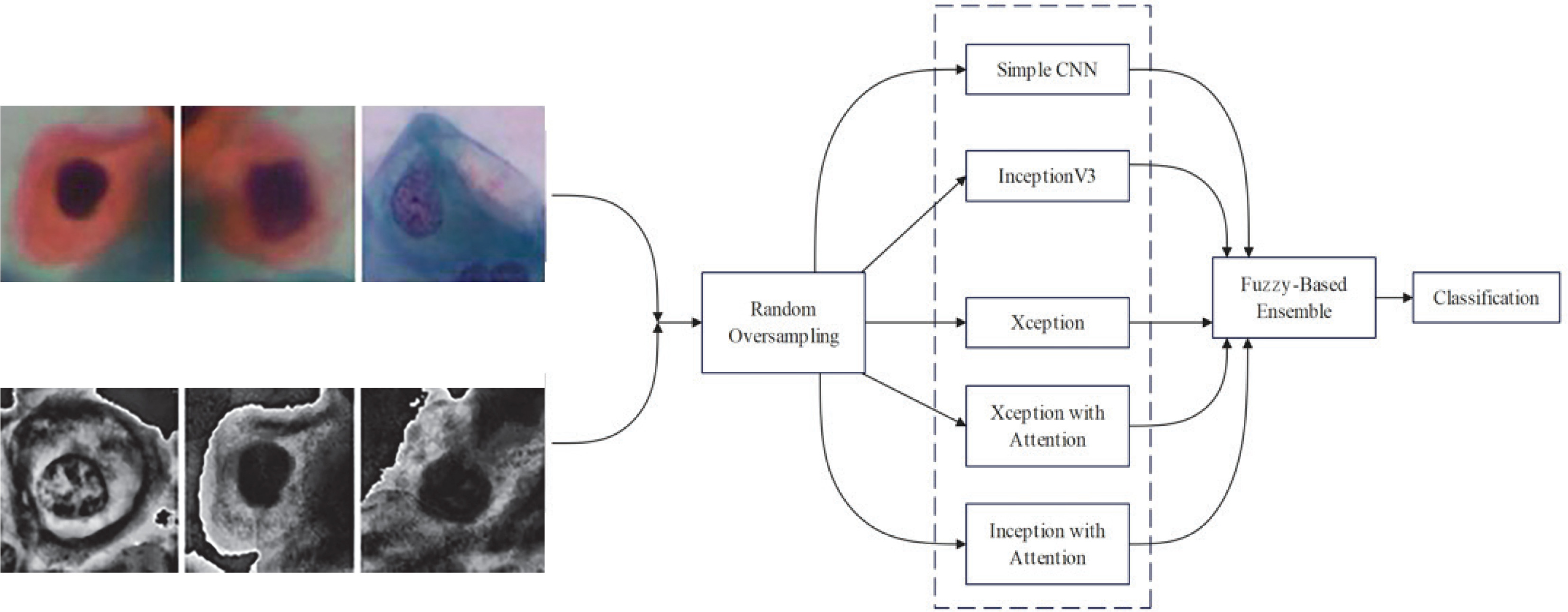
This section introduces the suggested method for cervical cell identification by utilising photographs from the dataset. The dataset was converted into a pre-processed version using pre-processing methods, and then the picture classes are by random oversampling. The new and original datasets without pre-processing are then input into 5 CNN models, including one basic CNN and 4 pre-trained CNN models. Among the 4 pre-trained CNN models, 2 include an attention mechanism. The attention method enables the model to concentrate on the most important picture regions, namely those likely to exhibit significant cervical abnormalities or cancer indicators. It is particularly important for Pap smear imaging because minor alterations in cell shape may indicate malignant or precancerous states. The attention mechanism selectively emphasises the most significant areas of the picture, enhancing the model’s efficiency and accuracy in detecting malignant cells or anomalies. This study examined 5 distinct CNN architectures from various origins to provide accurate assessments. InceptionV3 was chosen due to its parameter efficiency and enhanced performance in relatively sized datasets where its factorised convolutions minimise computation without compromising accuracy. Xception, on the other hand, replacing normal convolutions with depth-wise separable ones, performs better with fewer parameters in large datasets. Confidence ratings are obtained from each of the trained CNNs and aggregated via a fuzzy distance-based ensemble technique. A conclusive class is determined using 3 distinct distance metrics for contradictory data (i.e. disparate base classifiers provide divergent predictions). Figure 4 illustrates the flow diagram of the model, while Figure 5 depicts the whole pipeline of the suggested methodology.
Simple CNN
A convolutional neural network is a deep learning model applied mainly to image processing and computer vision tasks. Inspired by the human visual system, it contains 3 primary kinds of layers: convolutional layers for extracting features from images, pooling layers for down-sampling to reduce spatial dimensions while preserving important features, and classification is done through fully connected layers, also known as dense layers. The parameters used for designing the model are described in Table 1.
Table 1
List of parameters
InceptionV3
InceptionV3 is a deep CNN used to efficiently extract features and improve classification performance. It has a few inception modules, each of which contains several parallel convolutional branches: factorised convolution, asymmetric convolutions, and auxiliary classifiers.
This will reduce computation cost from O(n2k2) to
Auxiliary classifiers – During training the auxiliary classifier is used to provide an additional loss term
Ltotal= Lmain+ 0.3Lauxiliary , where Lmain is loss of the main classifier, Lauxiliary is loss of the auxiliary classifier, and 0.3 is th eweight of auxiliary loss.
Xception
Xception is a type of deep convolutional neural network (CNN) architecture introduced by François Chollet in the year 2017. It extends the inception architecture by fully substituting conventional convolutional layers with depth-wise distinct convolutions, making the model computationally efficient while retaining high performance. Xception decomposes the standard convolution into 2 independent processes: depth-wise convolution, which uses one filter per input channel, and pointwise convolution (1 × 1 conv), which combines the results of depth wise convolution with a 1 × 1 convolution. This helps to reduce the computational cost and improves learning efficiency but still allows for independent feature extraction. There are 3 key components of the Xception model: entry flow (extracts low-level features using depth-wise distinct convolutions), middle flow (deep feature extraction using repeated depth-wise distinct convolutions), and exit flow (final aggregation of features and classification).
The core innovation of Xception is the depth-wise distinct convolution, which replaces standard convolutions. For a standard convolution, the output feature map at position (i, j, k) is computed as Eq-9
where Wm,n,c,k is the filter weight, xi+m,j+n,c is the input feature map, F is the kernel size, C is the input channels, and bk is the bias term for output channel k.
However, in a depth-wise distinct convolution, there are 2 convolutions:
where Dm,n,c is the depth-wise filter
Point-wise convolution (1 × 1 convolution) – a 1 × 1 convolution combines the depth-wise output across channels, as per Eq-11
where Pc,k is a point-wise filter.
This reduces the number of multiplications from
Inceptionv3 and Xception with attention
The attention mechanism is used here to enhance the feature extraction from the model. To apply the attention, the feature map is reshaped into a sequence: F′ = Reshape(F)→(49,2048) . This transformation flattens spatial dimensions into a sequence of 49 vectors, each with 2048 channels. After this, the model applies multi-head self-attention to improve the representation of features, as per Eq-12:
where Q = F'WQ is the query matrix, K = F′WK is the key matrix, V = F′WV is the value matrix and dk is the scaling factor to stabilise gradients. The proposed model uses 8 attention heads – the attention function is applied 8 times in parallel and then concatenated as per Eq-13; this allows the model to attend to different spatial features simultaneously.
After this, Gaussian noise is added as a regularisation technique to improve generalisation, as shown in Eq-14 – this prevents the overfitting.
where noise is sampled from 0 to 0.25.
Ensemble model fuzzy-based distance
The suggested ensemble technique fuzzy-based distance is predicated on the notion that the deviation between recorded and optimal solutions must be minimised. In this context, the recorded solution denotes the confidence scores produced by various models for a specific sample, while the ideal solution signifies a confidence score of 1, reflecting absolute accuracy in categorisation. To quantify this difference, the consensus measure using 3 distance metrics has been calculated – Euclidean distance, Manhattan distance, and Cosine distances. These distance-based measures help in evaluating how close each classifier’s prediction is to the ideal case, ensuring a more robust and reliable decision-making process. Algorithm-2 outlines all the steps of the proposed method. There are 2 steps used by the ensemble process:
Direct agreement check – if all base classifiers unanimously predict the same class, that class is directly assigned as the final prediction.
Fuzzy distance-based aggregation – if classifiers provide varying predictions, the ensemble aggregates the confidence score using fuzzy weighting based on computed distances.
Let f = {(f1,c1),(f2 ,c2 ),− − −,(fm,cm)} be the dataset, where each sample fi ∈Rn belongs to a class ci ∈{1, 2,−−, n} , where n=5. Let j
For each sample fi and class label j , the ensemble is built by computing the distance between the confidence scores and the ideal solution vector
Algorithm-2 Fuzzy distance-based aggregation
Input – original dataset, CATEGORIES=”im_Dyskeratotic”, “im_Koilocytotic”, “im_Metaplastic”, “im_Parabasal”, “im_Superficial-Intermediate”
Output – performance metrics and predictions
Begin
**Define Function: compute_distances(feature_vector)**
**Define Function: get_final_prediction(distances)**
**Define Function: extract_features(image)**
**Define Function: preprocess_cervical_image(image_path, save_path, category_name)**
- Load image in grayscale mode.
- IF image is NULL:
- PRINT “Error: Image not loaded” and RETURN None.
- Apply **Wavelet Denoising** using Haar wavelet.
- Apply **CLAHE (Contrast Enhancement)**.
- Apply **Background Correction** using Morphological Opening.
- Apply **Edge Enhancement** using Laplacian filter.
- Save processed image with category prefix.
- Extract features from processed image.
- RETURN ‘final_save_path’, ‘feature_vector’.
**Define Function: fuzzy_aggregation(distances)**
- Initialize ‘final_scores’ as an empty dictionary.
- FOR each category in ‘distances’:
- Initialize ‘combined_score’ as an array of ones (for 5 classes).
- FOR each model:
- Compute **fuzzy weight** using product rule:
- Apply exponential transformation to sum of distances.
- Multiply ‘combined_score’ by fuzzy weight.
- Store the category with maximum aggregated score.
- RETURN ‘final_scores’.
**Define Function: process_all_images()**
- Initialize ‘final_predictions’ as an empty dictionary.
- FOR each category in ‘CATEGORIES’:
- Define paths for cropped images and ground truth storage.
-Create directories if not exist.
- FOR each image file in cropped folder:
- Check if file is an image.
- Call ‘preprocess_cervical_image ()’ to process the image.
- IF processed image or feature vector is None, CONTINUE.
- Compute distances using ‘compute_distances ()’.
- Predict final category using ‘get_final_prediction()’.
- Store prediction in ‘final_predictions’.
- RETURN ‘final_predictions’.
**Main Execution**
End
The work has considered 3 distance measures; therefore, 3 separate ensemble values are obtained: Euclidean-based ensemble
Application of Euclidean, Manhattan, and Cosine distances as fuzzy aggregators draws from their complementary characteristics in handling classifier confidence scores:
Euclidean distance quantifies the closeness in geometry between the predicted vector and the closest output in terms of total magnitude difference.
Manhattan distance looks at absolute value difference in terms of each dimension and hence is immune to outliers and extreme differences.
Cosine similarity encodes directional coherence between prediction vectors in terms of angular displacements instead of magnitude.
The ensemble system’s utilisation of all 3 measures takes advantage of the multiplicity of similarity viewpoints, hence making the system robust to cope with discordant predictions and stabilising classification. The product rule comes into play when considering the final fuzzy score to aggregate such measures so that models having greater agreement (i.e. closer to the solution optimum) are given greater weight.
To integrate the information obtained from distance measures, the product rule in Eq-17 is applied to each class label
The final prediction is made based on the selection of the class with the minimum aggregated distance as per Eq-18.
where ŷi represents the predicted class for sample fi. The product rule acts as a fuzzy measure, ensuring robust de-fuzzification by normalising distance values into a unified scale.
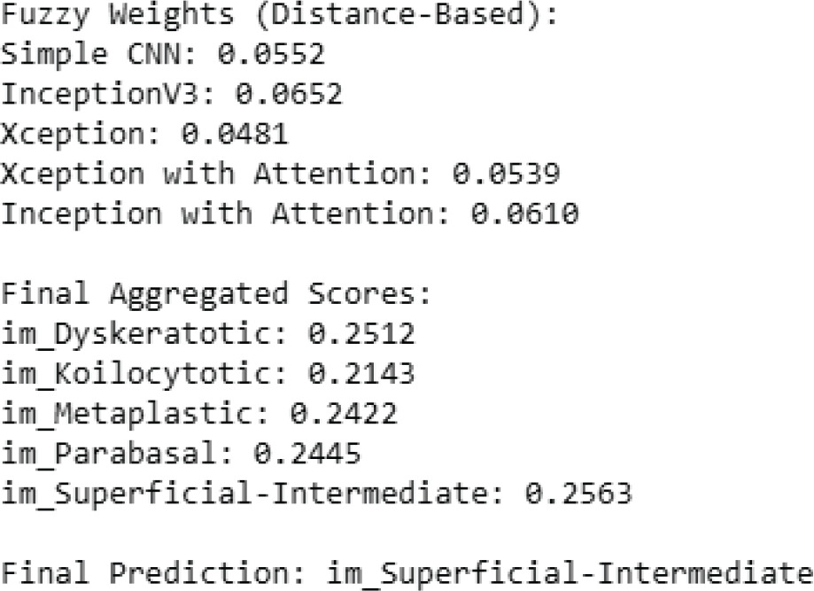
The sample example of the proposed approach by taking a sample fi (100 images) is presented in Figure 6, the best distance calculated for each base classifier is displayed, and accordingly the fuzzy aggregated score for each category is calculated by the proposed method and then displayed. The final prediction is done from the values of aggregated scores.
Results and Discussions
The model was simulated in python 3.x, using a Jupyter notebook with the machine having a main memory of 16 GB, GPU of 4 GB, and 8th Generation Intel Personal Computer (PC) [28]. An open-source dataset of Pap smear images was utilised to train and validate the model. The 5 deep learning models (simple CNN, InceptionV3, Xception, InceptionV3 with attention, and Xception with attention) were employed for the study. The models were trained in 2 stages. At the initial stage, the 2 models were trained and tested on the original Pap-smear dataset, and performance parameters were collected. At the final stage, the models were trained and tested on a newly created dataset formed by applying 4 pre-processing methods. Table 1 lists all the parameter settings used at the time of experiment.
Evaluation of framework with original dataset
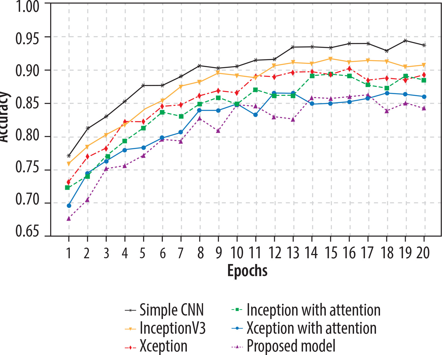
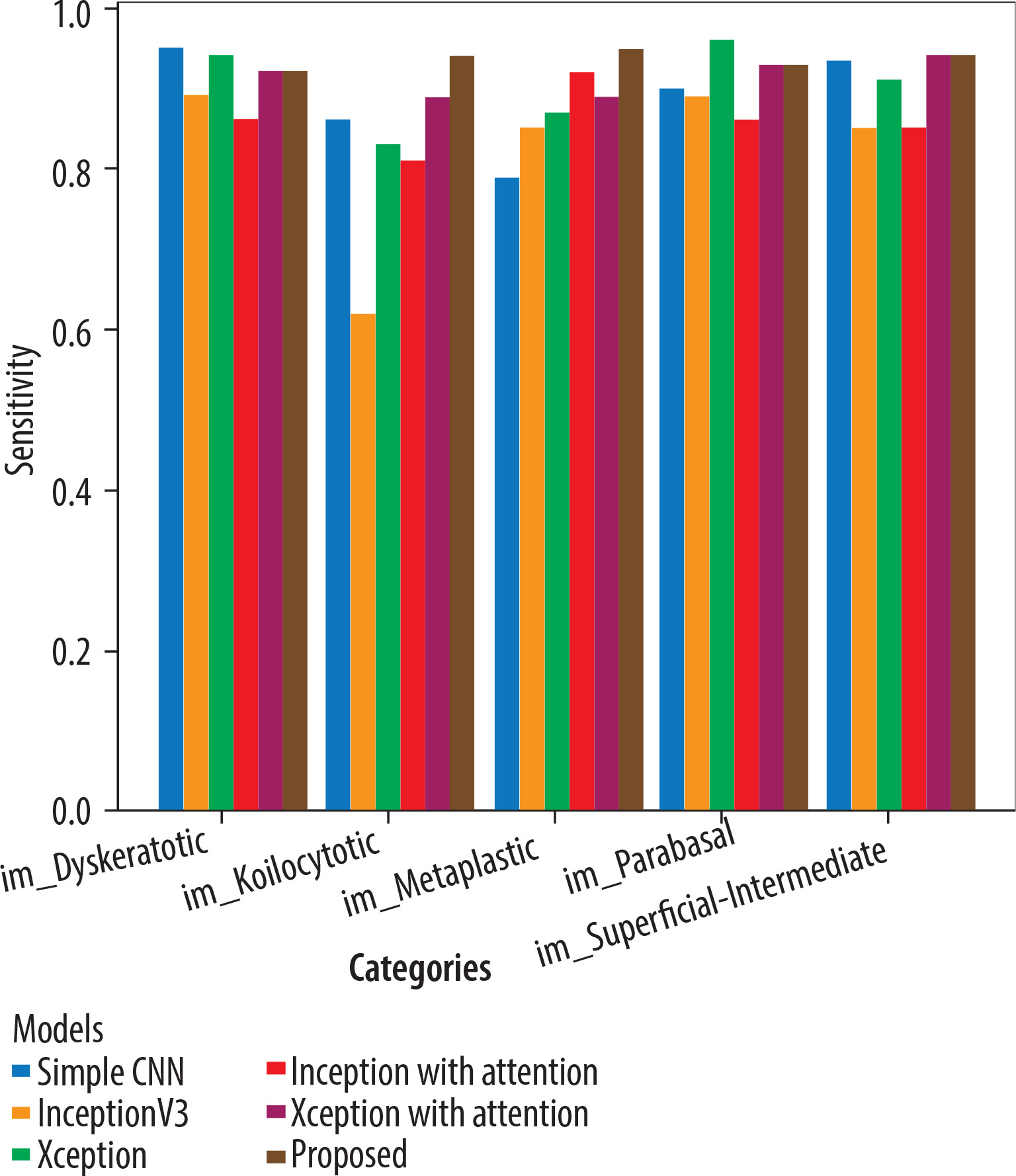
The Adam optimiser dynamically adjusts the learning rate during training, while the sparse categorical cross-entropy measures the difference between the predicted and the actual probabilities in the target dataset. All 5 models underwent training for 20 epochs. Xception with attention outperformed as a standalone feature extractor. After that, the proposed model was applied, and using the fuzzy aggregator method the score found to be 0.94. 80% of the original picture dataset was utilised in training the models, and the remaining 20% was used for validation. Accuracy and loss metrics were then generated for all the models. Simple CNN achieved an 87% average accuracy, Inceptionv3 achieved an average accuracy of 89%, Xception achieved an average accuracy of 90%, Inception with attention achieved an 86% average accuracy, Xception with attention achieved 92% average accuracy, and finally the proposed model achieved 94% accuracy. The model-wise performance metrics are listed in Table 2. For cervical cytology grading, recall is most critical. It directly contributes to patient outcomes by making sure the abnormal and pre-cancerous cells do not remain undetected, preventing delayed diagnosis and treatment. Figure 7 shows the accuracy comparison plot of the models, and Figure 8 is the recall plot of comparison of all the methods with the original dataset.
Evaluation of framework with new dataset
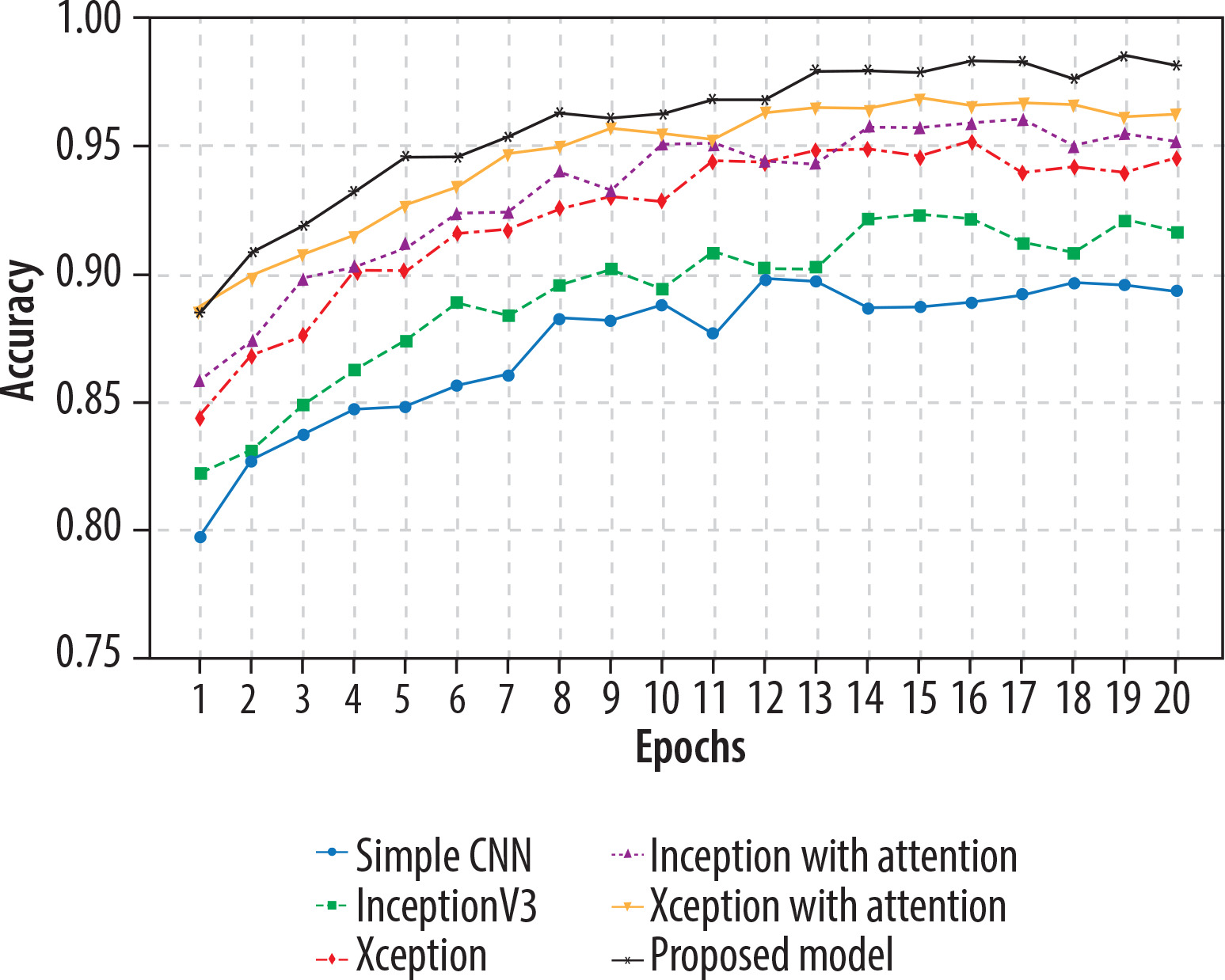
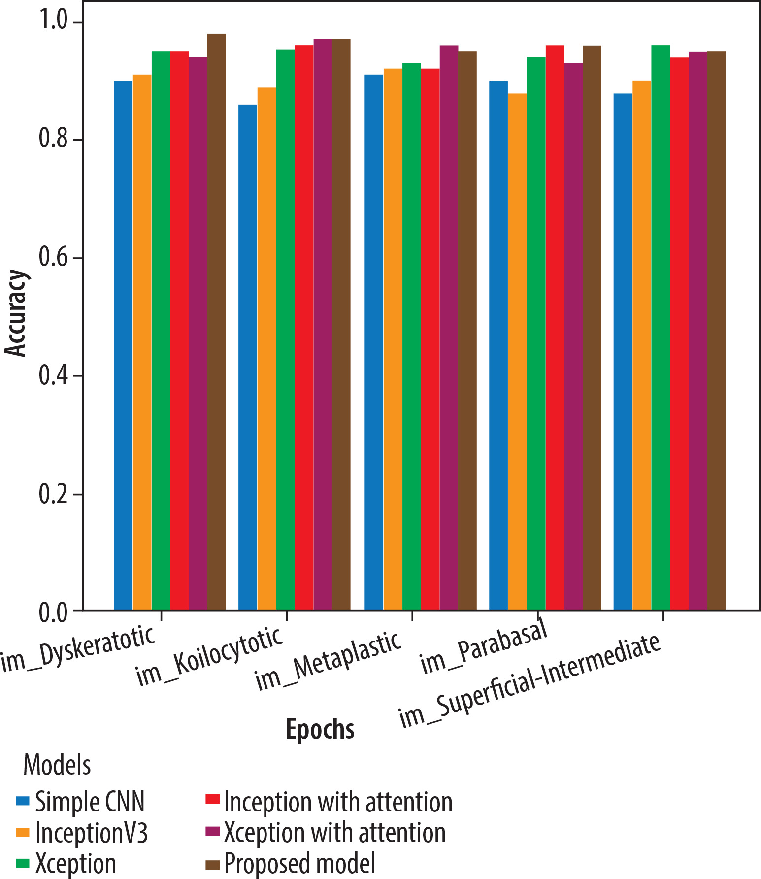
This section describes the evaluation of the models. All 5 models were trained on 20 epochs. Xception outperformed a standalone feature extractor. 80% of the new image dataset was utilised to train the proposed models, and the remaining 20% was used for validation. Loss and accuracy metrics were generated for all the models. Simple CNN achieved an 90% average accuracy, Inceptionv3 achieved an average accuracy of 92%, Xception achieved an average accuracy of 95%, Inception with attention achieved an 96% average accuracy, Xception with attention achieved 97% average accuracy, and the proposed model achieved 98.3% average accuracy. Figure 9 shows the plots of validation accuracy for each model, and other metrics including accuracy are listed in Table 3. Figure 10 is the recall plot of comparison of all the methods with the new dataset.
Performance comparison
Table 4 gives a comparison with previous work. The suggested fuzzy distance-based aggregation model outperforms all the previous methods, with 98.3% accuracy, compared to the best literature model (~92%). It also has the better recall (97.8%), which is more important in medical diagnosis. The attention-augmented models (Xception + Attention, Inception + Attention) are much better than their base counterparts, indicating the effect of incorporating self-attention in feature extraction. All the suggested models have been validated by SIPaKMeD, Herlev, or small datasets with the possibility of overfitting. The approach presented herein was trained on a large dataset with high generalisation capacity. Combining various models enhances the confidence in decision-making, the highest reported accuracy, recall, and F1 score for cervical cancer classification.
Table 4
Performance comparison with existing studies
| Study [Ref.] | Model | Dataset used | Data balancing | Accuracy | Precision | Recall | F1-Score |
|---|---|---|---|---|---|---|---|
| [24] | DenseNet-201 (Best among 13 CNNs) | Herlev Dataset | No | 87.02% | None | None | None |
| [27] | CervixNet (Digital Twin Approach) | SIPaKMeD Dataset | No | 91.30% | None | None | None |
| [29] | AlexNet, InceptionV3, ResNet-101, ResNet-152 | SIPaKMeD Dataset | No | ~85-90% | None | None | None |
| [33] | CNN + Transfer Learning | SIPaKMeD, Herlev | No | 89.50% | None | None | None |
| [35] | ResNet-18 + Random Forest | Real-world dataset | No | 90.50% | None | None | None |
| [37] | InceptionV3 + DenseNet201 | SIPaKMeD, Herlev | No | 92.00% | None | None | None |
| Proposed work | Simple CNN | Original Dataset | Yes | 87% | 0.872 | 0.87 | 0.866 |
| InceptionV3 | 89% | 0.9 | 0.905 | 0.87 | |||
| Xception | 90% | 0.92 | 0.94 | 0.93 | |||
| Inception + Attention | 86% | 0.9 | 0.9 | 0.87 | |||
| Xception + Attention | 92% | 0.91 | 0.93 | 0.92 | |||
| Fuzzy Aggregation | 94% | 0.93 | 0.94 | 0.923 | |||
| Proposed work | Simple CNN | New Dataset | Yes | 90% | 0.923 | 0.917 | 0.92 |
| InceptionV3 | 92% | 0.9 | 0.905 | 0.87 | |||
| Xception | 95% | 0.96 | 0.956 | 0.945 | |||
| Inception + Attention | 96% | 0.96 | 0.95 | 0.94 | |||
| Xception + Attention | 97% | 0.978 | 0.97 | 0.972 | |||
| Fuzzy Aggregation | 98.3% | 98% | 0.978 | 0.976 |
Conclusions
This Paper proposes a comprehensive approach for cervical cancer classification from Pap smear images based on CNN-based architectures, pre-trained deep learning models, and attention. The 5 models employed in the methodology are Simple CNN, InceptionV3, Xception, InceptionV3 with Attention, and Xception with Attention, and it concludes with a fuzzy distance-based aggregation function for overall classification. The experimental outcome indicates that the inclusion of the attention mechanisms greatly improves the model’s performance, with Xception + attention having higher accuracy than the baseline model. Secondly, the proposed fuzzy aggregation approach results in 98.3% improved accuracy, which is higher than previously in the literature. Of the measures tested, recall was found to be the most critical, facilitating correct identification of cervical cancer cases and avoiding false negatives, which is very important in medical diagnosis. In comparison to previous methods, the model described herein has better generalisability, avoiding the dataset limitations and overfitting problems experienced in previous studies.
Future deployment considerations and clinical translation
Although the presented ensemble architecture demonstrates superior classification performance, actual clinical deployment in practice encounters some problems. Five attention-enhanced CNNs form the existing framework, which, although it enhances accuracy and robustness, does so at massive computational expense. This could restrict its use in low-resource or point-of-care environments. To counter this, future research will explore model compression methods, such as pruning, quantisation, and knowledge distillation, to yield efficient yet lightweight versions of the ensemble.
Scalability is also a factor, especially in scaling the system to multi-centre datasets with diverse image types and acquisition protocols. Interoperability and standardisation will be enabled through pre-processing pipelines and adaptive learning modules, which will be essential.
For clinical validation, we partner with clinical centres to implement multi-site trials using prospectively collected data, representative populations, and real-world heterogeneity. Model explainability would also be improved through the embedding of Grad-CAM visualisations in clinical interfaces, enabling clinicians to better comprehend model predictions. These actions will enable regulatory clearance, clinician adoption, and integration into diagnostic pipelines.