Introduction
Tuberculosis (TB), caused by the bacterium Mycobacterium tuberculosis, is a highly infectious disease that primarily targets the lungs but can also affect other organs such as the kidneys, spine, and brain. The disease spreads through airborne particles expelled when an infected person coughs, sneezes, or talks, contributing to its high transmissibility. This study presents a novel approach to improving TB detection by leveraging chest X-ray (CXR) image datasets. The proposed method, TbCNN-net, integrates semantic segmentation with an adaptive convolutional neural network (CNN) architecture to enhance diagnostic precision. An India “TB Report 2024” by the Ministry of Health and Family Welfare reported estimated TB case numbers of 27.8 lakhs with 25.5 lakh in 2024, showing an increase from 24.2 lakh cases in 2023. There are various factors of risk of TB like undernourishment, diabetes, use of alcohol, HIV, smoking, etc. Ahmed et al. [1] introduced TB U-net with an attention mechanism for efficient segmentation of lungs. They also proposed a densenet-169 CNN for accurate classification of TB, COVID-19, and pneumonia. Nafisah [2] proposed TB detection by using 9 different CNN models with U-net segmentation and EffcientNetB3, achieving higher accuracy of 99.1% with receiver operating characteristic (ROC) of 99.9%, recall of 98.8%, precision of 98.8%, and f1_score of 98.8%. Also, it involved different visualisation techniques like Grad-CAM and t-SNE [3]. Sharma et al. [4] proposed an U-Net model for segmentation with accuracy of 96.35%, Jaccard index of 90.38%, and DCE coefficient of 94.88%, and a classification model of Xception with accuracy of 99.29%, precision of 99.30%, and recall of 99.29%. They also used Grad-CAM to show the heatmap pattern and developed a framework with 9 different CNN models, among which CheXNet was the best performing model with accuracy of 96.47%, sensitivity of 98.56%, precision of 98.57%, and f1_score of 98.56%. Rajaraman et al. [5] trained X-rays using a U-Net model on TBX11 CXR dataset. Shallow models like VGG16 and VGG-19 were used for classification with staple consensus region of interest for region localisation on Montgomery TB and Shenzhen TB datasets [6]. This study trained and evaluated 10 different deep CNNs for distinguishing TB cases from normal cases. The models included ResNet50, ResNet101, ResNet152, InceptionV3, VGG16, VGG19, DenseNet121, DenseNet169, DenseNet201, and Mobile Net. The approach presented here leverages histogram-matched CXR images, eliminating the need for object segmentation of regions of interest. This approach enhances the accuracy and detection performance of CNN models for TB identification by incorporating histogram matching with CXR images. Chavan et al. [7] proposed Res-UNet++ outperformed U-Net and Res Net architectures, achieving superior evaluation metrics, including a validation Dice coefficient of 96.36%, validation mean IoU of 94.17%, and validation binary accuracy of 98.07% [8]. A novel algorithm has been developed to refine segmented masks, enhancing final accuracy, alongside an efficient fuzzy inference system for more weighted activity assessment. Dao and Lin [9] gives a comparison between U-Net, UNet++, and TransUNet+ [10]. ConvNet achieved sensitivity 87.0%, f1-score of 87.0%, 88.0% precision [11]. The algorithm achieved outstanding performance in detecting pulmonary tuberculosis (PTB), with an area under the receiver operating characteristic curve (AUC) of 0.878 and a 95% confidence interval (CI) ranging from 0.854 to 0.900 in the NTUH-20 dataset [12]. Swin ResuNet3 was used for segmentation of images, and a Multi-scale Attention-based DenseNet with an Extreme Learning Machine model was used for classification of TB [13]. An attention block integrating VGG16 and VGG19 architectures is employed for classifying TB CXRs. In the study by Verma et al. [14], a deep learning model was proposed for TB diagnosis, incorporating deep learning features alongside Gabor and Canny edge detection in one approach, and excluding these techniques in another, achieving accuracies of 95.7% and 97.9%, respectively [15]. Le et al. [15] used 5 pretrained models: VGG16, EfficientB7, MobileNetV3, DenseNet121, and RegNetY040 for classification of TB, among which MobilenetV3 showed the best performance with an accuracy of 98.35%, f1-score of 98.32% on TB CXR, Montgomery accuracy of 77.81%, and f1-score of 78.92%, and on the Shenzhen dataset – an accuracy of 67.19% and f1-score of 74.86%, on the India CXR – accuracy of 86.25% and f1-score of 83.75%.
Material and methods
Datasets and preprocessing
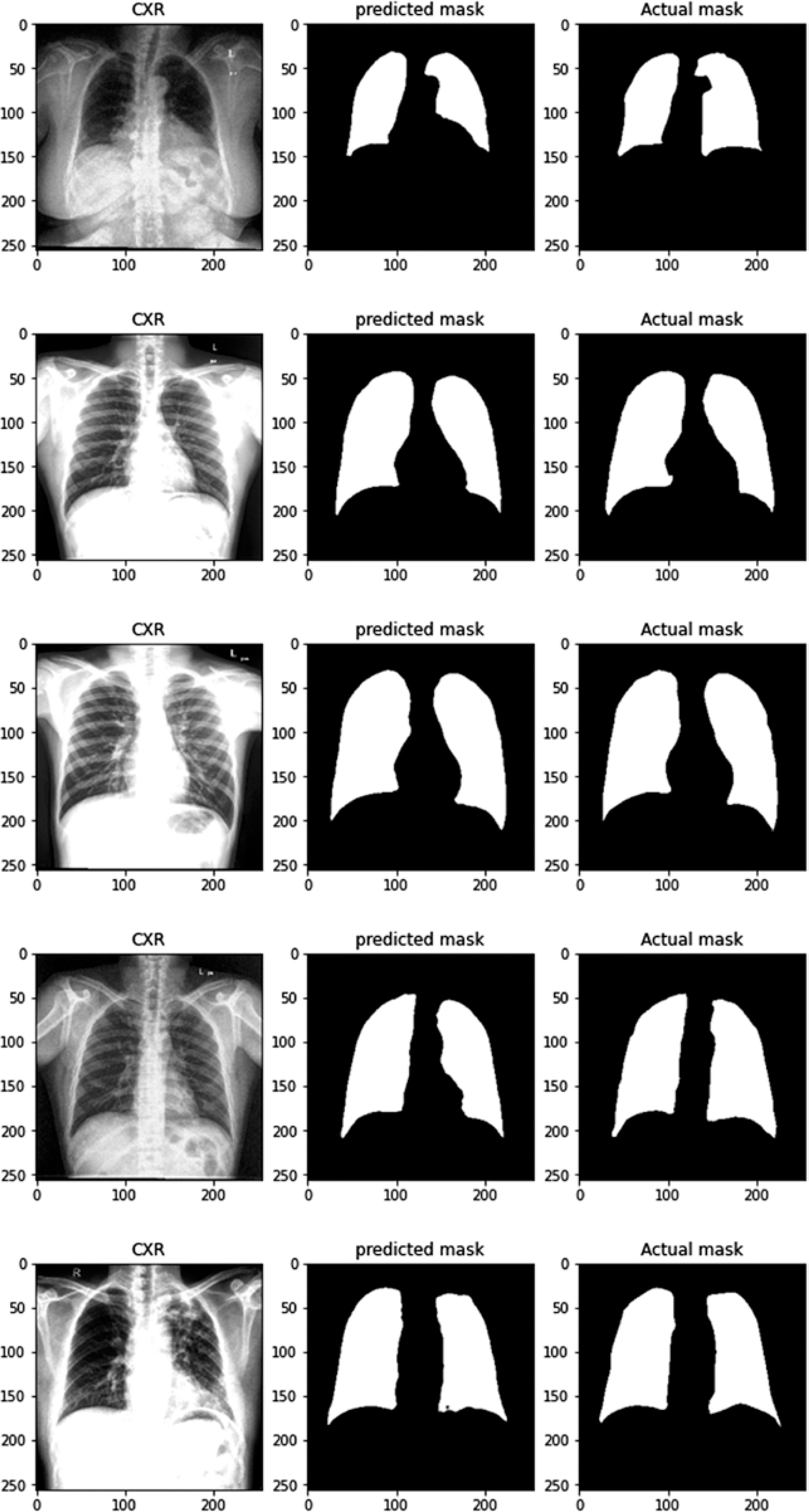
For the segmentation task, we utilised the Montgomery County and Shenzhen Hospital datasets, both obtained from the publicly available “Chest X-ray Masks and Labels” dataset on Kaggle. The combined dataset comprised 704 CXR images, each paired with corresponding segmentation masks. The data was split into 494 images (70%) for training, 140 images (20%) for validation, and 70 images (10%) for testing. To ensure a robust evaluation, we implemented a five-fold cross-validation strategy, allowing each image to be used at least once for both training and testing. For the classification task, we used the “National Institute of Allergy and Infectious Diseases (NIAID) TB Portal Program” dataset, which is part of the “Tuberculosis Chest X-ray Images” dataset on Kaggle. This dataset included 700 CXR images of TB patients and 3500 control images. For our experiment, we selected 700 TB images and 700 control images, which were divided into 1120 images (80%) for training, 140 images (10%) for validation, and 140 images (10%) for testing. Figure 1 shows sample images from this dataset.
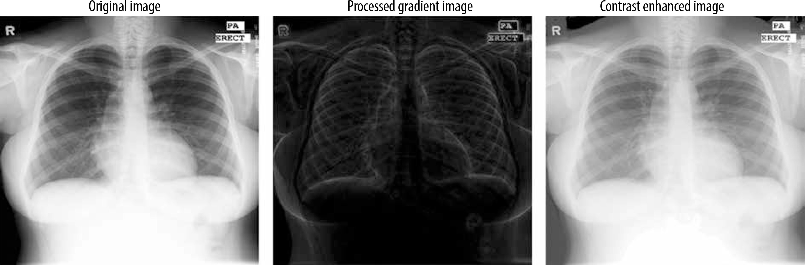
Before being input into the model, the images were normalised by scaling the pixel values to a [0, 1] range, achieved by dividing each pixel by 255. This normalisation process ensures uniformity across the dataset, optimising the model’s training performance. Also a gradient based contrast enhancement technique with gamma correction is used (Figure 2).
Methods
Figure 2 outlines the methodology employed in this study. We started by selecting a well-established chest X-ray (CXR) dataset, which included both the images and their corresponding segmentation masks for training the segmentation model. Before segmentation an enhanced gradient based technique for contrast enhancement was used.
Enhanced gradient-based contrast enhancement technique with gamma correction
The gradient computation function captures intensity changes by comparing each pixel with its neighbours in 4 directions, emphasising edge-like features. Pyramid reduction processes the image at multiple resolutions to capture gradients at different scales, mimicking multi-scale edge detection. Unique mapping and histogram matching adjust pixel values based on gradient information, enhancing contrast by redistributing intensities. Finally, gamma correction (with a value of 0.5) boosts brightness in darker regions, further improving contrast.
Steps for enhanced gradient-based contrast enhancement:
Take the original image as input and show the original image in greyscale.
Reduce the resolution by the cv2.pyrDown() function and perform padding and gradient initialisation.
Do gradient computation by padding the input image, traversing each pixel, extract a 3*3 sub image, and compute the differences between the centre pixel and its neighbours.
The gradients for original and reduced images should be computed at multiple levels.
Perform normalisation of the gradient by ensuring a minimum value and computing the geometric mean.
Display gradient-based images.
Unique mapping and histogram matching.
A final contrast image is created and displayed.
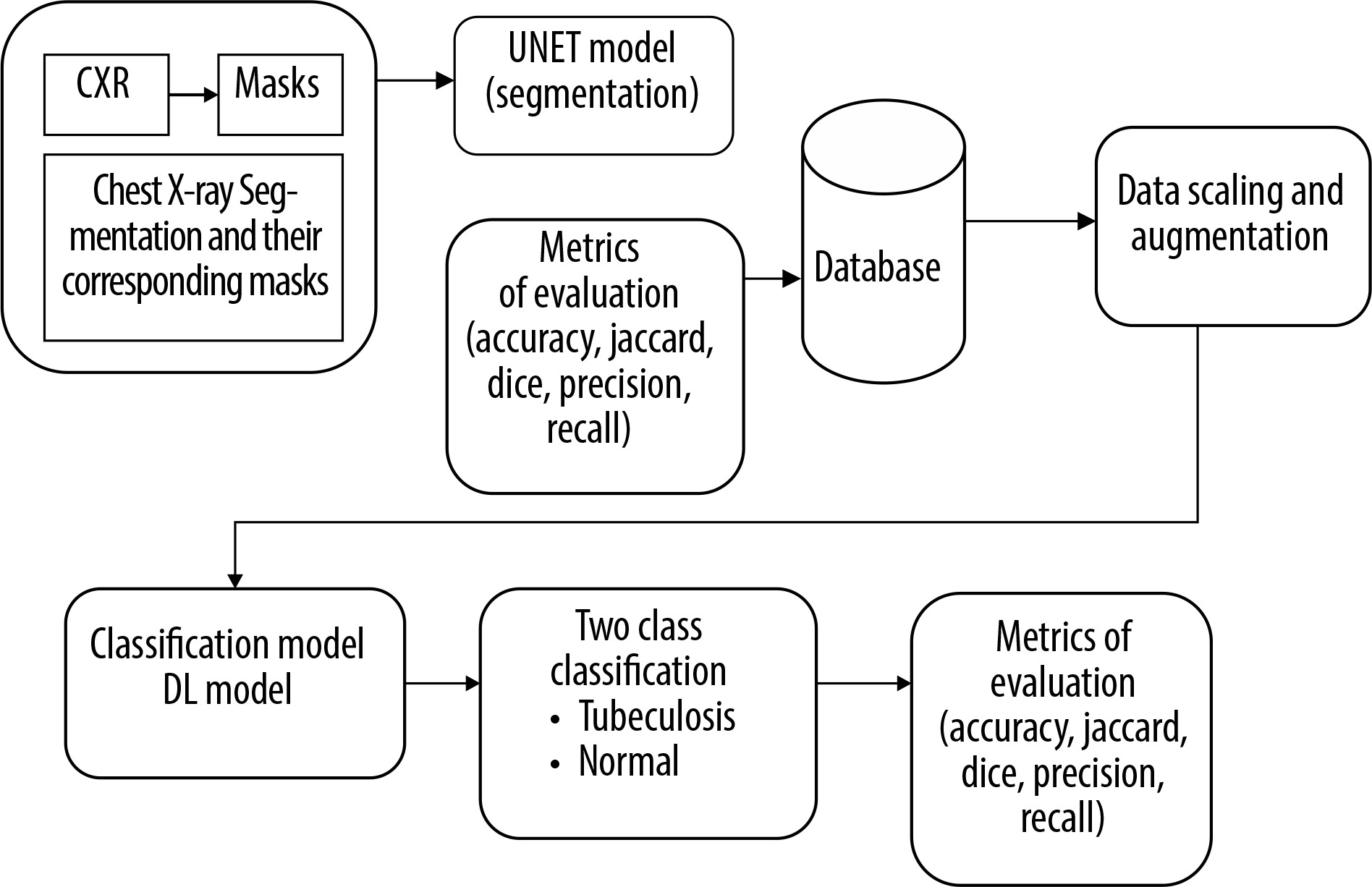
Next, we modified and optimised the model to improve its performance. The process began with the selection of a well-established CXR dataset, which included both images and their corresponding segmentation masks, for training of the segmentation model. The U-Net architecture, a popular model for segmentation tasks, was modified and optimised to align with the study’s objectives. The performance of the trained segmentation model was assessed using metrics such as accuracy, Dice coefficient, Jaccard index, and AUC. The model was then applied to CXR datasets containing both TB and normal cases to segment the lung regions while excluding background information. Following segmentation, a deep learning CNN was developed and fine-tuned to classify the segmented lung images. The classification model’s performance was evaluated using various metrics, including accuracy, precision, recall, F1-score, AUC, and ROC curves.
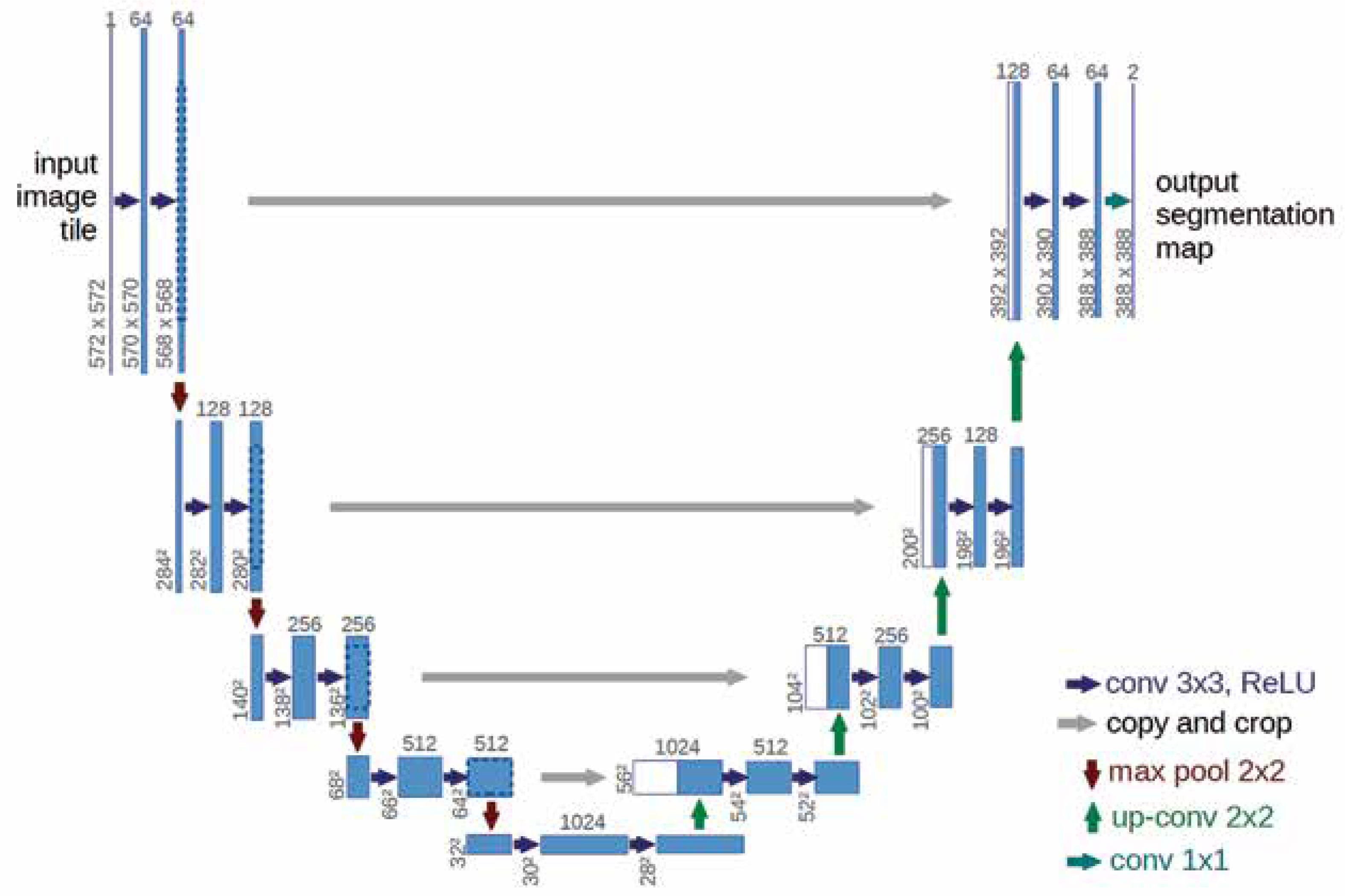
U-Net model (segmentation model)
The U-Net model is a widely recognised and highly effective architecture for image segmentation, particularly in medical applications such as segmenting organs, tissues, or lesions in medical scans like CT, MRI, and CXR. It was originally designed for bio-medical image segmentation but has since become widely adopted for various segmentation tasks. Originally developed by Olaf Ronneberger in 2015, U-Net has become one of the most popular and effective models for segmentation tasks in medical imaging, especially for analysing radiological images.
Figure 3 illustrates the U-Net architecture, which comprises 2 main components: the encoder and the decoder. The encoder employs a sequence of convolutional layers combined with ReLU activation and max-pooling operations. Conversely, the decoder reconstructs segmented images using up-convolution layers, depth concatenation, softmax activation, and max pooling. The process starts with a 224 × 224 pixel input image, which is processed by the encoder to extract features represented as numerical values between 0 and 255. These values are normalised to a scale of 0 to 1. As the image progresses through the encoder, its dimensions decrease after each max pooling operation. A bridge channel links the encoder and decoder, facilitating the transfer of extracted features. The decoder reconstructs the image by interpreting these numerical values, assigning pixel values below 0.5 to 0 and those equal to or greater than 0.5 to 1. Skip connections between the encoder and decoder enable the direct transfer of image features, ensuring minimal information loss during neural node processing. The decoder’s final output comprises binary images with pixel values of 0 (black) and 1 (white), producing black-and-white masks that emphasise regions of interest, such as the lung area in CXR. The U-Net model was trained for 50 epochs per fold, using a learning rate of 0.001 and a dropout rate of 0.25. The batch size was set to 4 images per batch for both training and validation. The cross-entropy loss function, LCE, is expressed as:
where i represents the index of the sample (e.g. image), and yi is the ground truth label, with yi = 1 for the positive class and 1 – yi = 0 for the negative class (Figure 4).
Modified U-Net model
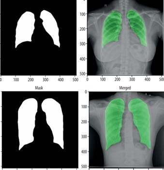
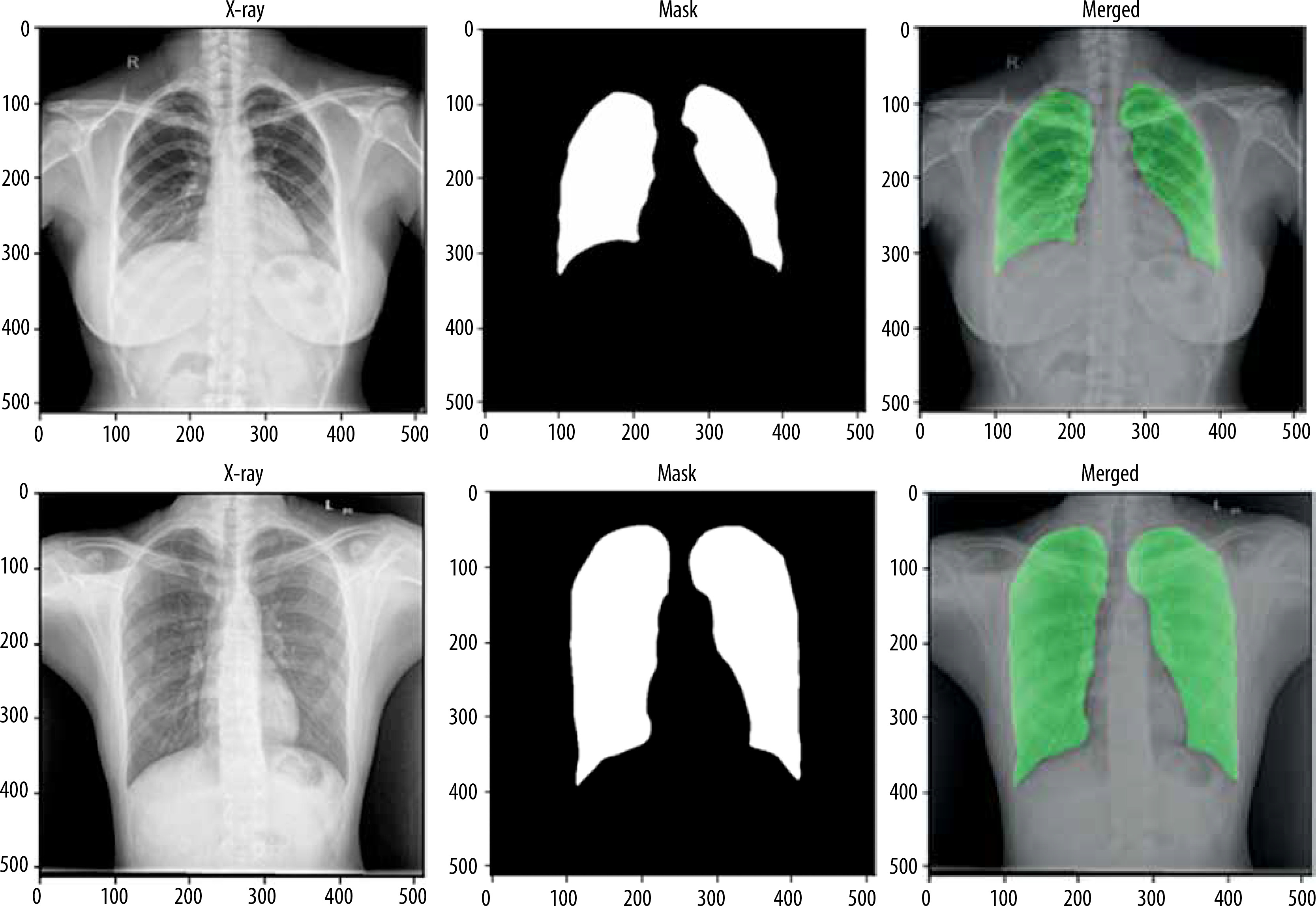
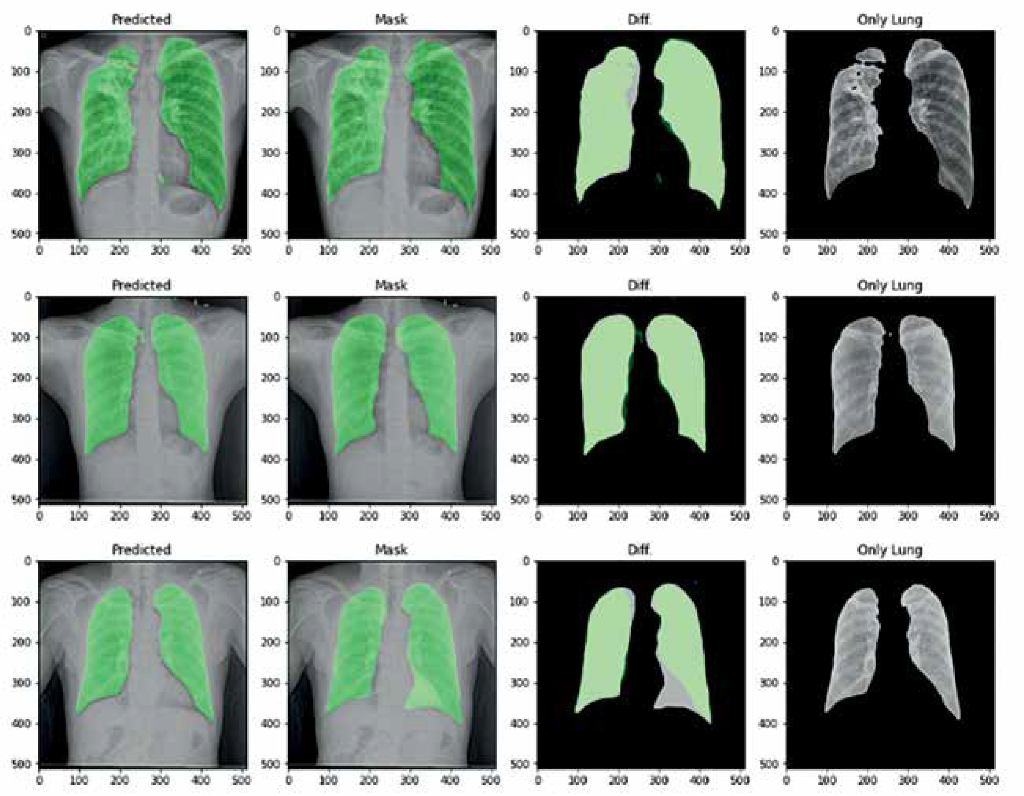
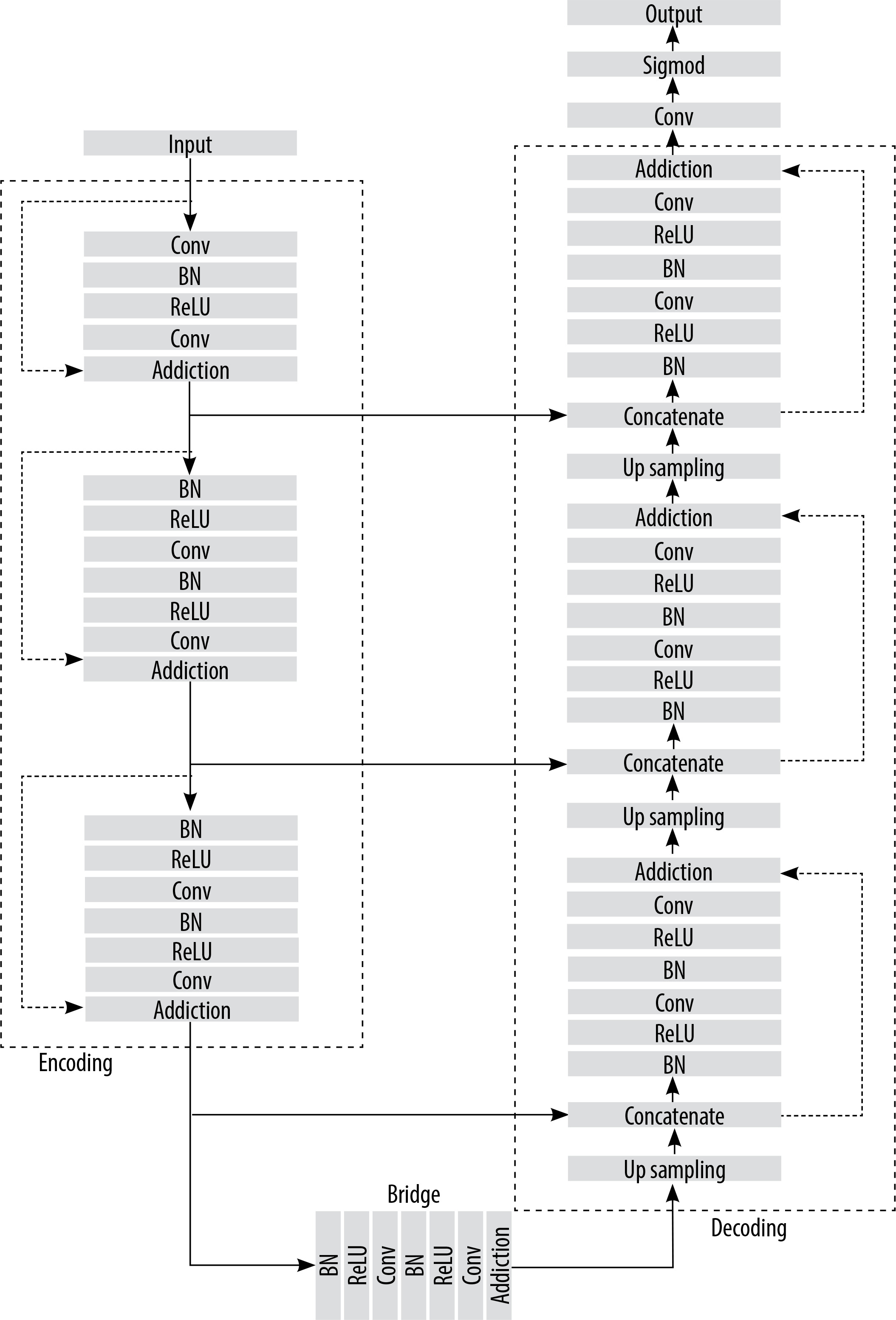
For lung image segmentation, the researcher adopted a deep learning approach using U-Net with residual connections. U-Net, developed by Olaf Ronneberger et al. for biomedical image segmentation, can be further optimised by replacing standard convolutional units with residual units. Figure 5 shows the architecture of the residual U-net Network. U-Net (ResU-Net) combines the advantages of both U-Net and residual neural networks to achieve better segmentation. results. The ResU-Net architecture is designed to simplify network training while preserving information flow through its skip connections in residual units, preventing degradation. It consists of 3 key components: encoding, bridge, and decoding (Figure 5). Figure 6 illustrates chest Xray images with actual and predicted masks from Res-Unet model
Classification model
The classification model employs a CNN architecture specifically designed for image classification. It processes input images through multiple convolutional layers that extract hierarchical features, with each layer followed by max pooling. The convolutional layers detect localised patterns and features, while max pooling reduces spatial dimensions, enhancing computational efficiency and feature abstraction. The features extracted by these layers are then flattened into vector representations and passed through multiple fully connected (dense) layers to complete the final classification. These dense layers enable the model to capture complex features.
The equation for the dense layer is given below:
where x – the input vector or tensor, W – the weight matrix, b – the bias vector, σ – the activation function applied elementwise, y – the output of the dense (fully connected) layer.
The output layer employs the sigmoid activation function (as shown in Equation 3) to estimate the probability of the input image belonging to a specific class.
Hybrid model
The hybrid model enables the simultaneous segmentation and classification of input images by leveraging the strengths of both approaches. First, the segmentation model identifies and generates masks that highlight specific regions or objects within the image. The segmentation masks are subsequently input into the classification model, which conducts binary classification using the segmented regions. This approach allows the model to integrate global context with localised details, improving its capability to identify the presence or absence of specific features in the image. The model employs the binary cross-entropy loss function and the Adam optimiser to ensure efficient learning across both segmentation and classification tasks. The accuracy metric further highlights the model’s effectiveness in executing both tasks with precision. This hybrid approach provides a flexible and reliable solution for complex image analysis, particularly in scenarios requiring continuous segmentation and classification.
TBNet-CNN model
The proposed TBNet-CNN model integrates a segmentation model and a classification model into a single hybrid architecture, as illustrated in Figure 7. The process for developing and training this hybrid model using Tensor flow and Keras is detailed in Algorithm 1. The segmentation component is initially defined, consisting of convolutional layers for feature extraction and up-sampling layers to generate segmentation masks. Next, the classification model is defined, incorporating convolutional and dense layers specifically designed for image classification tasks. These 2 components are then integrated to form the hybrid model. The model is trained using labelled data, with training data used for model construction and validation data for performance monitoring.
Input: Input shape = (256, 256, 3)
Define the segmentation model
1. Initialize input layer:
inputs ← Input (input_shape)
2. First convolutional layer:
convolution1 ← Conv2D(32, (3, 3), activation=’relu’, padding=’same’)(inputs)
3. Max pooling layer:
pool1 ← MaxPooling2D(pool_size=(2, 2))(convolution1)
4. Upsampling layer:
up1 ← UpSampling2D(size=(2, 2))(pool1)
5. Final convolutional layer for mask generation:
decoded ← Conv2D(3, (3, 3), activation=’sigmoid’, padding=’same’)(up1)
6. Define segmentation model:
segmentation_model ← Model(inputs, decoded, name=’segmentation_model’)
Define the classification model
1. Initialize input layer:
inputs ← Input(input_shape)
2. First convolutional layer:
convolution1 ← Conv2D(16, (3, 3), activation=’relu’) (inputs)
3. Max pooling layer:
pool1 ← MaxPooling2D(pool_size=(2, 2)) (convolution1)
4. Second convolutional layer:
convolution2 ← Conv2D(32, (3, 3), activation=’relu’) (pool1)
5. Max pooling layer:
pool2 ← MaxPooling2D(pool_size=(2, 2)) (convolution2)
6. Third convolutional layer:
convolution3 ← Conv2D(64, (3, 3), activation=’relu’) (pool2)
7. Max pooling layer:
pool3 ← MaxPooling2D(pool_size=(2, 2)) (convolution3)
8. Fourth convolutional layer:
convolution4 ← Conv2D(64, (3, 3), activation=’relu’) (pool3)
9. Max pooling layer:
pool4 ← MaxPooling2D(pool_size=(2, 2)) (convolution4)
10. Fifth convolutional layer:
convolution5 ← Conv2D(64, (3, 3), activation=’relu’) (pool4)
11. Max pooling layer:
pool5 ← MaxPooling2D(pool_size=(2, 2)) (convolution5)
12. Flatten the output:
flatten ← Flatten()(pool5)
13. First dense layer:
dense1 ← Dense(256, activation=’relu’)(flatten)Final
14. Output layer (sigmoid):
output ← Dense(1, activation=’sigmoid’)(dense1)
Combine the segmentation and classification models
1. Initialise input tensor:
input_tensor ← Input(input_shape)
2. Apply segmentation model:
segmentation_output ← segmentation_model(input_tensor)
3. Apply classification model:
classification_output ← classification_model(segmentation_output)
4. Create hybrid model:
hybrid_model ← Model(inputs=input_tensor, outputs=classification_output, name=’hybrid_model’)
Compile and train the hybrid model
1. Compile the hybrid model:
hybrid_model.compile(optimizer=’adam’, loss=’binary_crossentropy’, metrics=[‘accuracy’,’dice_coeff’,’jaccard_index’])
2. Define log directory for tensorboard:
logdir = ‘logs’
3. Train the model:
hist ← hybrid_model.fit(train, epochs=25, validation_data=val, callbacks=[tensorboard_callback])
Pseudo-code for TB detection system
The pseudocode in the proposed model section outlines the system’s workflow, including input processing, segmentation, classification, and the final output. The process begins with an input image of size 256 × 256 × 3, which is first processed by the segmentation model. This involves encoding the image using Conv2D and MaxPooling2D layers, followed by decoding with Upsampling2D and Conv2D layers to generate the segmented output. The segmented images are then passed to the classification model for further analysis. During classification, the images are processed through several Conv2D and MaxPooling2D layers, followed by a Flatten layer and 2 Dense layers to produce the final classification. This hybrid approach seamlessly integrates segmentation and classification, offering a robust solution.
Specify the input image shape:
Set the input shape to 256 × 256 × 256 (height, width, and RGB channels).
Construct the segmentation model:
Input layer: Establish the input layer for the model.
Encoder: Employ a series of Conv2D and MaxPooling2D layers to extract hierarchical features.
Decoder: Use UpSampling2D and Conv2D layers to recover spatial dimensions and refine the segmented output.
Output layer: Use a sigmoid activation function for pixel-wise binary classification.
Build the classification model:
Input layer: Define the input layer for the classification model.
Convolutional layers: Use a sequence of Conv2D and MaxPooling2D layers to extract important features.
Flatten layer: Flatten the feature maps into a 1D vector.
Dense layers: Use fully connected layers with Relu activation for complex feature interactions.
Output layer: Use a sigmoid activation function for binary classification.
Integrate the models:
Compile and summarise the hybrid model: Compile the hybrid model with a suitable optimiser and loss function, and generate a summary of its architecture.
Results
This section offers a detailed overview of the evaluation metrics employed to measure the performance of the TBNet-CNN model. These metrics are crucial for determining how effectively the model identifies patterns and makes predictions, serving as key indicators of its overall performance. Accuracy is a key metric for classification models, representing the ratio of correctly predicted instances to the total number of instances, providing an overall assessment of prediction reliability. Recall measures the model’s ability to accurately identify positive instances, which is especially important when detecting all positive cases is critical. The F1-score, which combines precision and recall into a harmonic mean, provides a balanced evaluation of the model’s performance, especially when both metrics are equally important or when dealing with imbalanced classes. Additionally, the confusion matrix offers a comprehensive breakdown of the model’s predictions compared to the actual ground truth labels, consisting of 4 key elements: false positives (FP), false negatives (FN), true positives (TP), and true negatives (TN). This enables a deeper analysis of the model’s predictive accuracy and error patterns. The equations for f1_score, recall, and precision are given below:
(7)
Loss curves and accuracy curves for pre-trained and TBCNN-net models are shown in Figure 8.
Figure 8
Loss and accuracy curves of different CNN models. A) Loss and accuracy curves for TBCNN-net. B) Loss and accuracy curves for VGG16. C) Loss and accuracy curves for DenseNet121. D) Loss and accuracy curves for VGG19. E) Loss and accuracy for ResNet50. F) Loss and accuracy curves for Xception
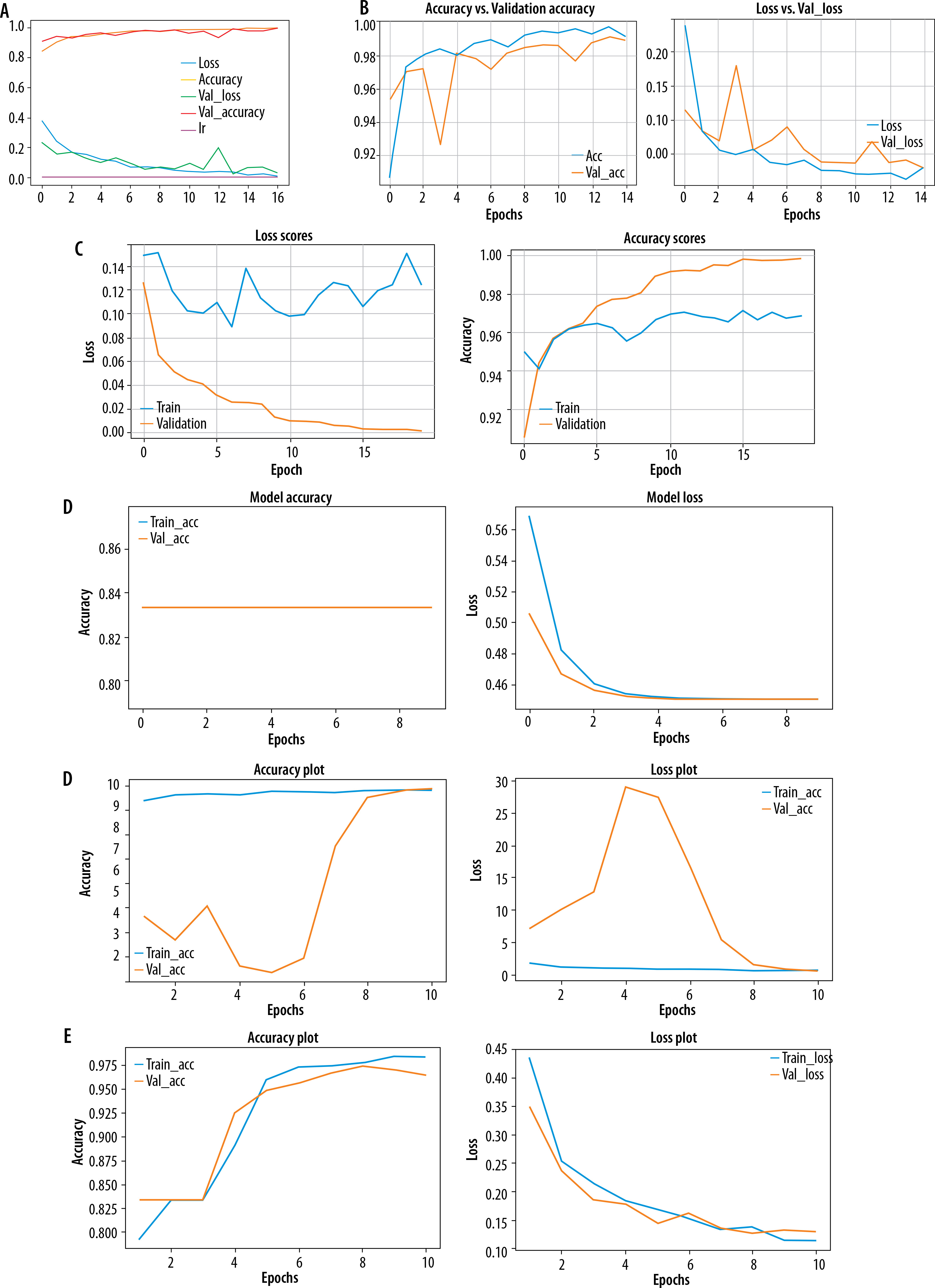
Tb-CNN net accuracy seemed to be higher than other pre-trained models, and the loss is also low compared to other models.
U-Net and Res-UNet loss and accuracy curves are shown in Figure 9. From this figure we can see that Res-UNet performs better than U-Net.
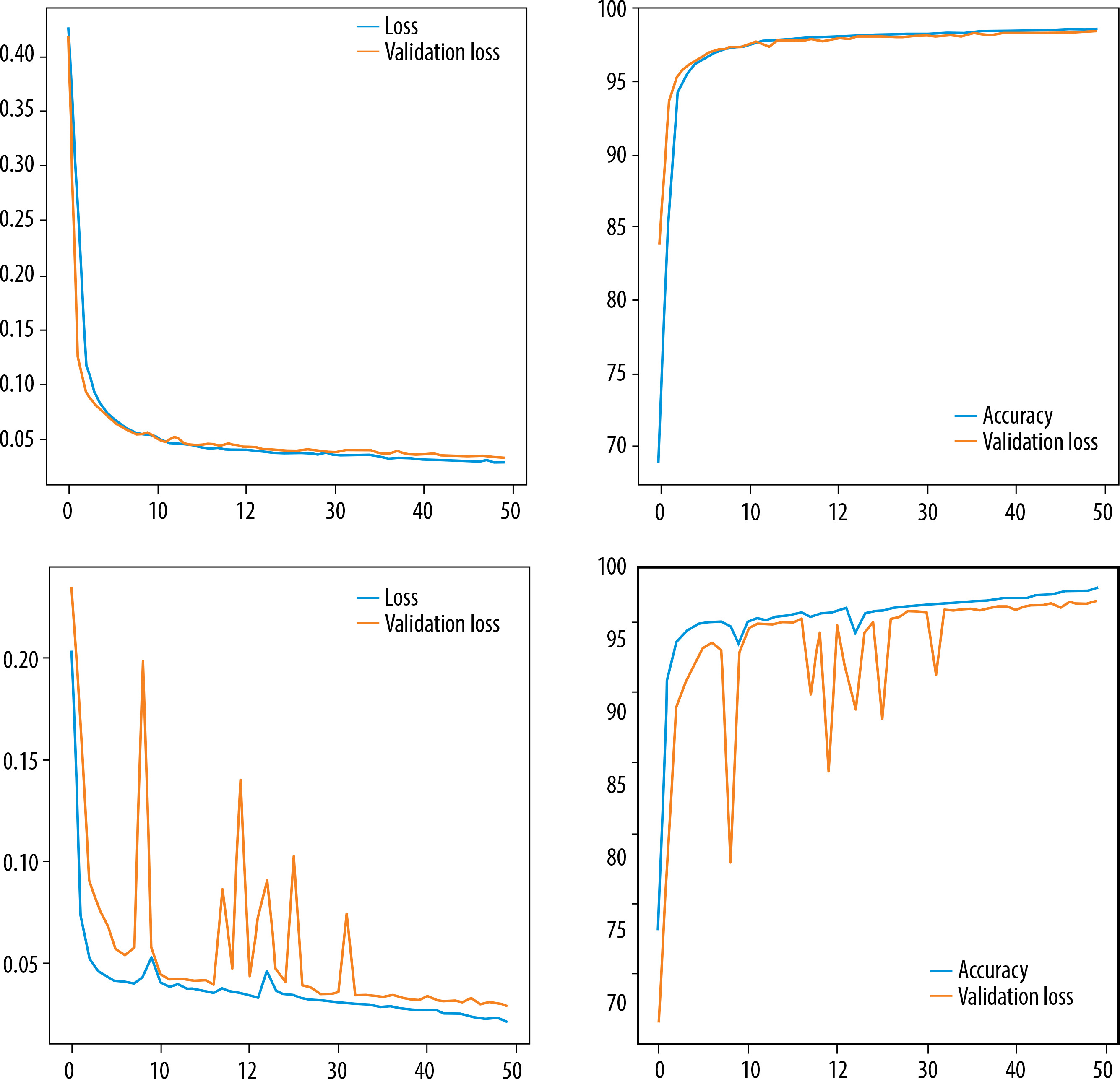
Table 1 shows the accuracy of ResUnet is 98.18, recall is 98.40, precision is 98.39 which is quite more as compared to that of Unet. Only f1_score and dice coefficient is little less. But on an average the performance of ResUnet is quite good as compared with Unet Model.
Discussion
Confusion matrices for TBCNN-net and other pretrained models are shown in Figure 10.
Figure 10
Confusion matrix of all pre-trained and TBCNN-net models. A) Confusion matrix of DenseNet121. B) Confusion matrix of InceptionV3. C) Confusion matrix of Xception. D) Confusion matrix of VGG16. E) Confusion matrix of VGG19. F) Confusion matrix of TBCNN-net. G) Confusion matrix of ResNet50
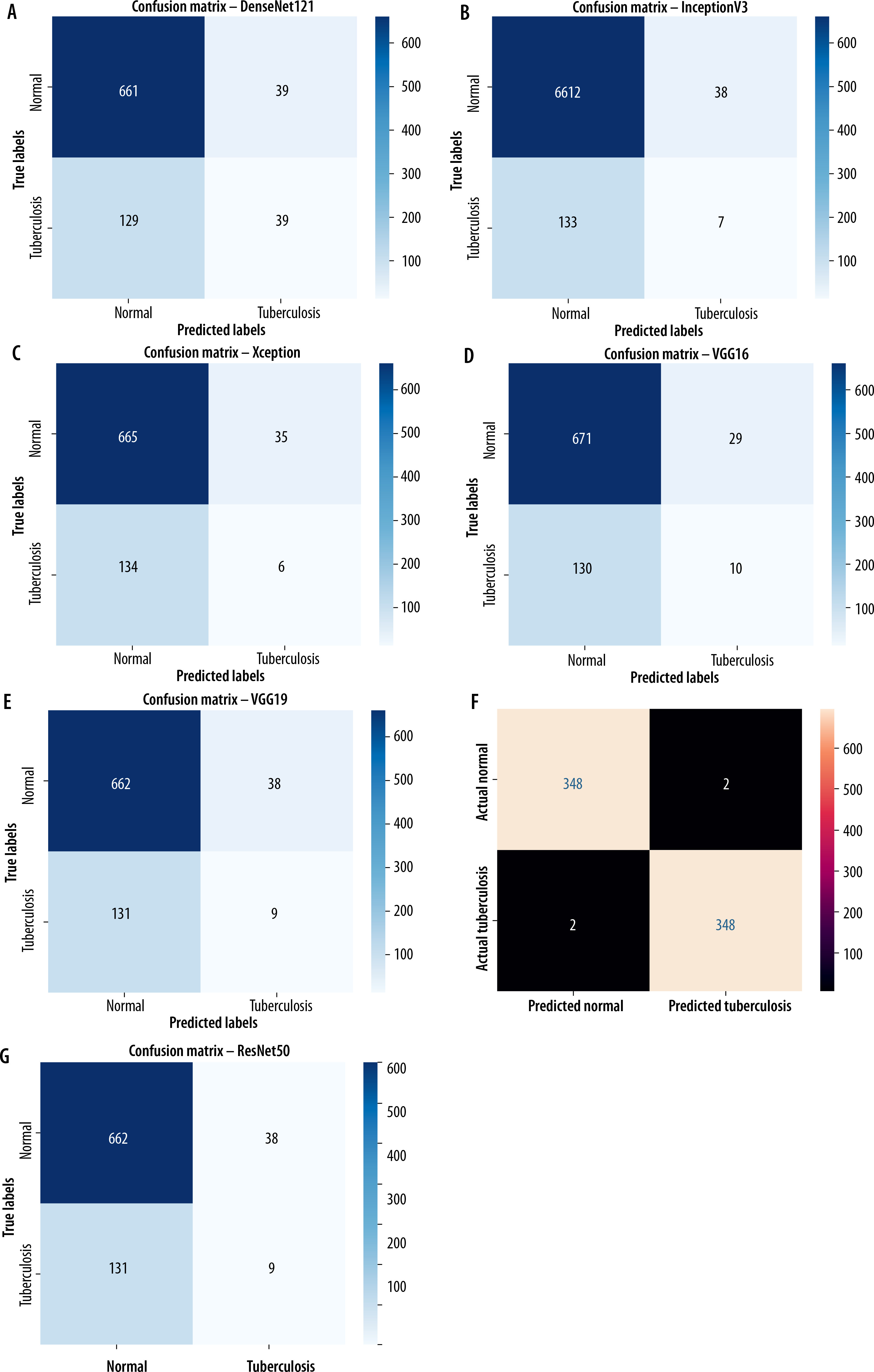
As compared to other pre-trained models, TBCNN-net performed with 348 predicted and actual TB cases, followed by DenseNet121 with 11, VGG16 with 10 cases, VGG19 with 9, InceptionV3 with 7, and Xception with 6 cases.
Table 2 shows that the TBCNN-net has the greatest accuracy.
Table 2
Metrics of performance between TBCNN-net and other pre-trained models
| Model name | Accuracy | Precision | Recall | f1_score |
|---|---|---|---|---|
| VGG16 | 81.35 | 55 | 52 | 50 |
| VGG19 | 80.59 | 51 | 51 | 49 |
| DenseNet121 | 80.24 | 53 | 51 | 50 |
| Xception | 79.65 | 49 | 50 | 48 |
| InceptionV3 | 79.17 | 49 | 50 | 48 |
| ResNet50 | 83.35 | 42 | 50 | 45 |
| TBCNN-net | 99.45 | 99.03 | 99.29 | 99.29 |
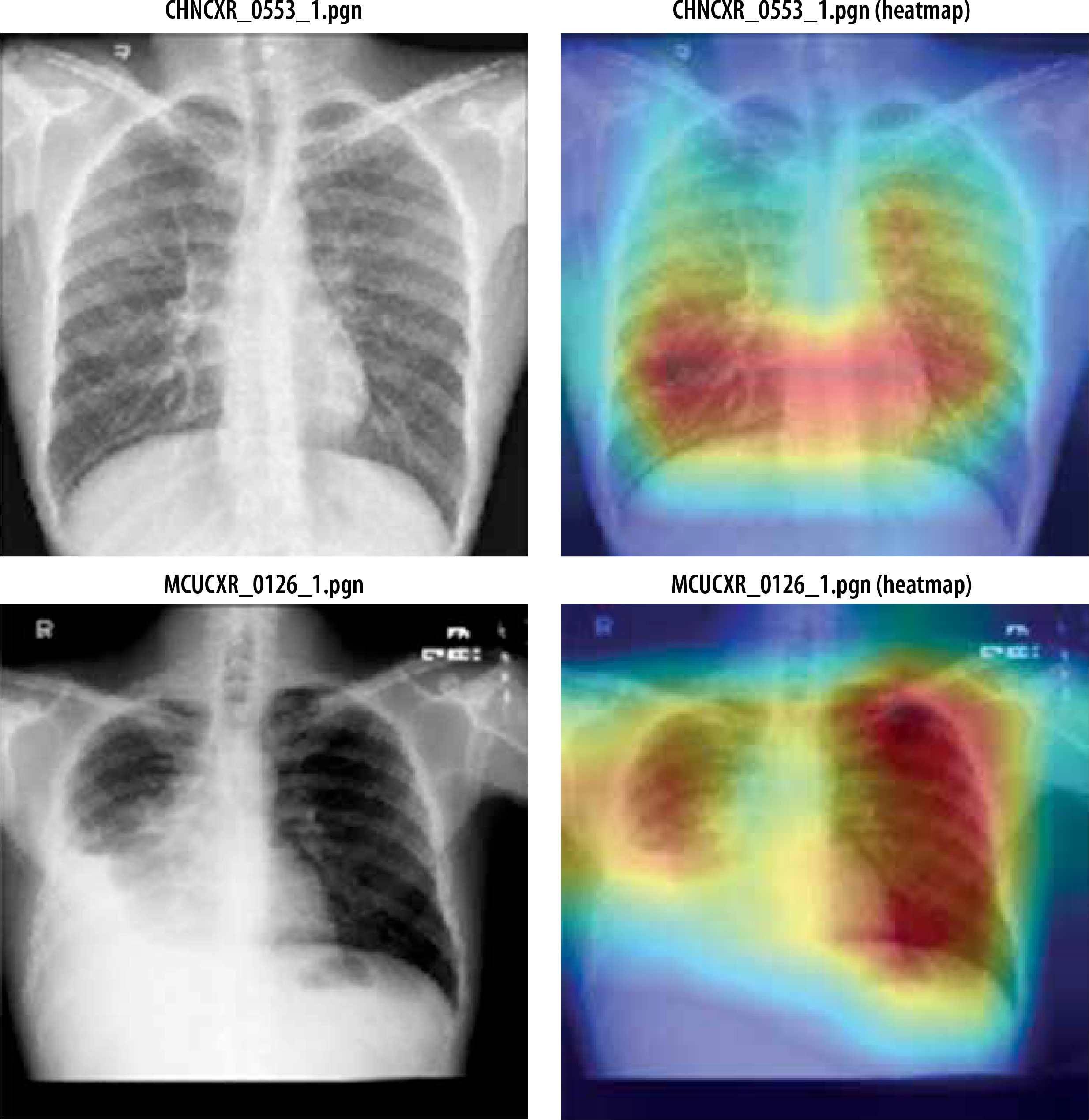
Figure 11 shows heatmap for segmented images indicating presence of disease infected regions.
Conclusions
This study introduces a novel deep learning-based CNN model, TBCNN-net, designed to detect TB from X-ray images. The model employs a two-stage architecture, combining a segmentation module with a classification module to enhance prediction accuracy. Comprehensive evaluations highlight the system’s reliability and practicality, outperforming previous methods in terms of accuracy of 99.45% and recall of 99.29%. Additionally, its superior Jaccard index of 96.05% and Dice coefficient of 96.33% further validate its performance using residual U-net architecture. When tested on unseen images, TBCNN-net demonstrated robustness and strong generalisation across diverse datasets, maintaining high accuracy. Future research will focus on integrating multimodal data, including genetic information and clinical metadata, to create more advanced diagnostic tools and deepen insights into it. TB detection values further validate its performance.