Introduction
Artificial intelligence (AI) is a computer science technology that has existed for more than 70 years [1]. From a technical point of view, it is a very broad group of digital solutions aimed at mimicking human intelligence. Today, AI has a wide range of applications in many aspects of daily life. The scope of these solutions extends from self-driving vehicles to stock market predictions, search tools, social networks, and as far as aerospace engineering [2].
Significant advancement in AI is also observed in medicine, where many tools in the AI domain are utilised [3,4]. Radiology, in particular, is a rich area for machine learning solutions, and the number of studies on AI in this field has been increasing year by year [5]. In 2015, Ronneberger et al. [6] published the first study on image segmentation, aiming to segment brain and cervical neoplasm cells on microscopic imaging examinations. The driving force behind the development of AI in radiology is the belief that AI can match physicians in diagnostic accuracy [7]. In the larger picture, it may help increase of the efficiency of radiology units, which face a constantly growing number of patients requiring diagnostic evaluation [8]. Furthermore, it is emphasised that AI is not subject to significant human nature disadvantages that the radiologist may present. AI does not become fatigued or distracted, and emotions do not influence the accuracy of its diagnoses [7].
Convolutional neural networks (CNNs) are a subset of machine learning methods and, more broadly, AI neural networks in which the main mathematical operation is convolution. They are applied in a variety of tasks, but their primary purpose is the analysis of images or series of images. In medicine, CNNs are used mainly in histopathology [9] and radiology [10], where their primary tasks include detection, classification, or derivatives of these operations.
The positioning of the patient during radiological examinations plays a crucial role in determining the diagnostic utility of the obtained results. Positioning errors sometimes result from improperly performed examinations, but most often are related to the patient’s condition and behaviour during the procedure [11]. In the case of X-ray images (radiographs) used to assess the presence of pathology, with some exceptions, at least two projections are usually required. Each projection is carried out in a precisely defined manner to encompass selected anatomical structures in their entirety and in well-defined geometric relationships. This allows the radiologist to easily and reliably identify abnormalities. On the other hand, an improperly taken X-ray image can lead to a misdiagnosis, which can have serious medical consequences. For example, improper alignment of the axis of the area being examined in relation to the image axis can lead to the superimposition of anatomical structures and, as a result, limit the interpreter’s ability to make a correct assessment.
The aim of our project was to develop a tool to assess the correctness of the axis of X-ray images of the ankle joint (AJ) in the antero-posterior (AP) and lateral (LAT) projections on properly taken radiographs. This assessment is the first step in the imaging diagnostic path that aims to obtain the accurate measurements necessary to plan the treatment of conditions such as degenerative changes or injuries to adjacent bone structures in the case of the AJ.
Our solution utilises CNNs to effectively assess the correctness of the analysed radiographs. To the best of the authors’ knowledge, this is the first work concerning the evaluation of the correctness of projection axes on standardised radiographs, especially in AJ imaging, according to guidelines and literature. The described experiments are the preliminary stage of the development of an automated imaging diagnostic system for AJ alloplasty procedures.
Material and methods
Dataset and projection correctness determination
For numerical experiments, a total of 1062 AJ X-rays defined as AP and LAT projections from the years 2015-2022 were used from the archives of the Department of Imaging Diagnostics of the University Hospital in Krakow. The above-mentioned AP group included 528 X-rays while the LAT group consisted of 534 pictures. Of these radiographs, 404 were assessed as invalid and the other 658 as valid.
The studies were randomly selected, without taking into account the characteristics of the patients such as sex, the side of the body examined, trauma history, osteoarthritic changes, internal stabilisation with metallic elements, or external stabilisation in the form of a plaster cast or other type of dressing.
The data were retrieved in the form of images saved in Portable Network Graphics (PNG) format due to the lossless compression applied in this format. Additionally, any markings by radiology technicians and any other elements that allowed the identification of the patient were removed from the images as part of the complete anonymisation of the data.
The projection correctness was determined based on Lampigiano and Kendrick [12] and the relevant literature containing angular measurements used for planning AJ alloplasty [13-16]. Four projection annotations were applied for AJ X-ray studies: AP, rotated AP (APr), LAT, and rotated LAT (LATr).
The true AP projection was defined as including the distal 1/3 of the fibula and tibia bones, the talus bone, and the proximal segments of the metatarsal bones. In this projection, the foot bones should not be rotated, and their anterior-medial aspects should be visible. The projection denoted APr is targeted at the distal tibiofibular syndesmosis (DTFS). This kind of view should be done in AP oblique projection with the foot tilted medially with an angle of 30-45 degrees and should include the distal 1/3 of the fibula and tibia bones, the talus bone, the calcaneus bone, and the base of the fifth metatarsal bone. Importantly, the APr projection should display the entire joint cavity of the upper AJ, a clearly visible distal tibiofibular joint space, and the medial malleolus with joint surface shadow overlap.
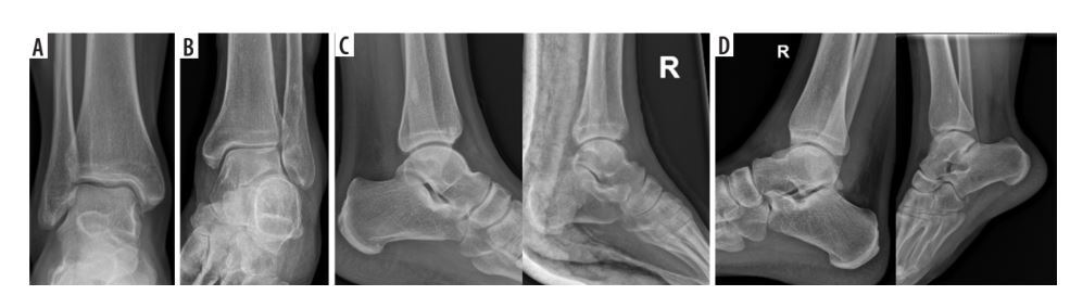
The other projection group consisted of two LAT projections. The LAT projection shows the distal 1/3 of the fibula and tibia bones, the LAT aspects of the talus bone, the calcaneus bone, the other tarsal bones, and the base of the fifth metatarsal bone. The foot should not be rotated in the vertical or horizontal axis, and the fibula bone should overlay the posterior half of the tibia bone. The most important difference between the standard LAT projection and the LATr projection is the presence of evident rotation in the form of the crossing of the arcs of the talus bone and/or the articular surface of the tibia bone in the shape of the letter “X”. It is worth noting that the slightly non-overlapping AJ joint surfaces which are approximately parallel or slightly shifted in the shape of “<” did not affect the angular measurements, and therefore the radiologist included them in the LAT group. The examples of projections assigned to the four groups AP, APr, LAT, and LATr are presented in Figure 1.
Figure 1
Projections of the antero-posterior (AP), rotated AP (APr), lateral (LAT), and rotated LA (LATr) groups. A) AP projection, without a visible tibiofibular syndesmosis gap. B) Oblique antero-posterior projection (APr), showing a clear tibiofibular syndesmosis gap and overlapping shadows of the medial malleolus with a straight line of the medial articular surface of the upper ankle joint. C) Two examples of correct LAT projections, with a slight horizontal axis deviation that does not affect angular measurements. D) Two examples of LATr, with the first image showing the crossing of the articular surface of the talus bone in an “X” shape, and the second image displaying significant horizontal axis rotation, creating a wide fan-shaped appearance resembling “<”
Architecture and hardware
The binary classification method was applied. The input of the system was a digital X-ray image saved in PNG format, and the output was a binary decision (valid or invalid) based on the input X-ray image. The database was divided into a training, validation, and test set, according to an 80 : 10 : 10 ratio. The model was developed using a training dataset (323 invalid images and 526 valid images) and was automatically evaluated on a validation dataset (40 invalid and 66 valid). The test set was used to assess the model performance under conditions similar to how the algorithm would be used in real-life applications. The test dataset included 66 images classified by an expert radiologist as valid and 41 images classified as invalid.
The model was obtained using a Python script accessible from GitHub [17] that searched through all possible Keras Neural Network structures, selecting the best one and retraining the selected structure. For the assessment of radiograms correctness, the Xception network containing CNN was chosen. Xception is known for its depth-wise separable convolutions, which are efficient for image recognition tasks. The computation time of Xception for training and evaluation was about 4 hours on a computer system equipped with a 30-core Intel Xeon Gold CPU and 360 GB of RAM. The experiments were carried out under the Linux openSUSE Tumbleweed operating system distribution.
Performance evaluation
The performance of the model was evaluated using binary classification metrics. The metrics used included accuracy, precision, recall (sensitivity), and the F1 score (equations 1-4). In each metric, the notation is understood as follows: TP – true positives, TN – true negatives, FP – false positives, FN – false negatives.
Results
Thirty-two neural networks were tested. Table 1 shows the results of the initial training through the search of the Keras Neural Networks.
Table 1
Results of initial training through the grid search of the Keras Neural Networks and accuracy for the validation set
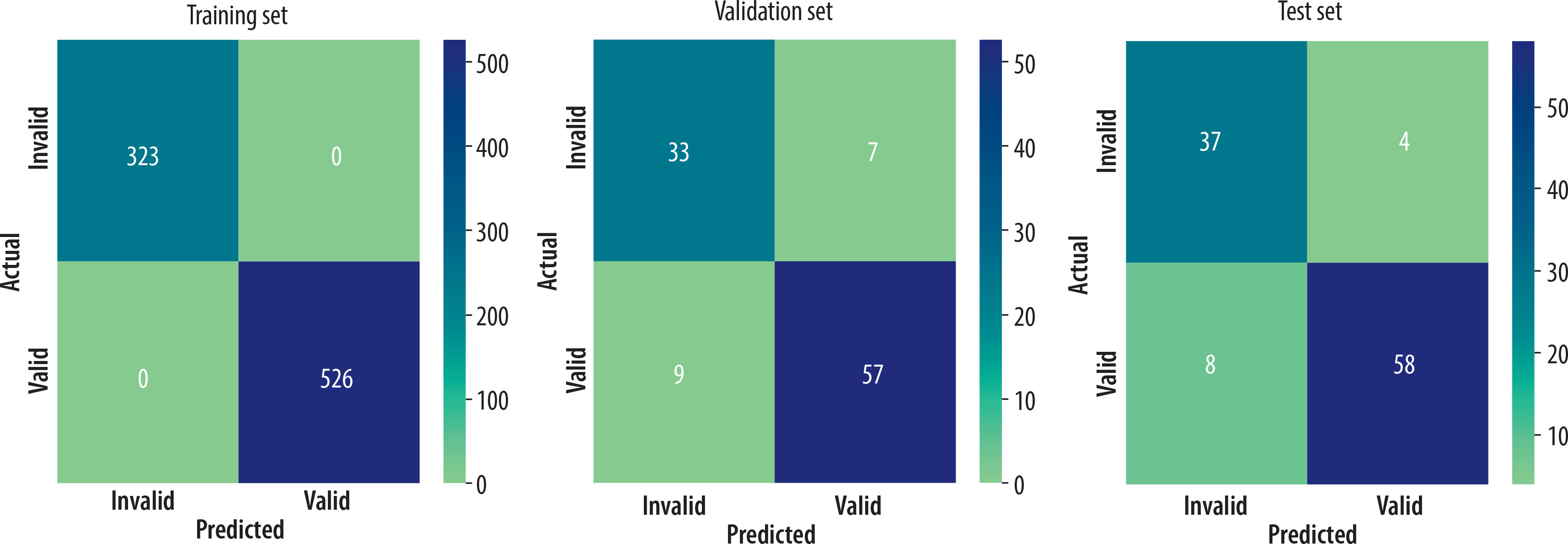
The optimal modified Xception architecture, selected among 32 evaluated neural networks, yielded accuracies of 1.0, 0.849, and 0.888 for the training, validation, and test sets, respectively. Table 2 shows the other metrics calculated for the chosen architecture and Figures 3A and 3B contain confusion matrices for each set.
Table 2
Results of classification metrics
| Dataset | Accuracy | Precision | Recall | F1 |
|---|---|---|---|---|
| Training | 1.000 | 1.000 | 1.000 | 1.000 |
| Validation | 0.849 | 0.891 | 0.864 | 0.877 |
| Test | 0.888 | 0.935 | 0.879 | 0.906 |
Figure 2
The architecture used for image classification is Xception, a deep convolutional neural network (CNN) architecture. The colours of the blocks correspond to different types of layers: blue – convolutional; violet – separable convolutional; orange – max pooling; yellow – global average pooling; and green – softmax [Graphics based on Westphal et al. A Machine Learning Method for Defect Detection and Visualization in Selective Laser Sintering Based on Convolutional Neural Networks’ with modifications. Additive Manufacturing 2021; 41. DOI: https://doi.org/10.1016/j.addma.2021.101965]
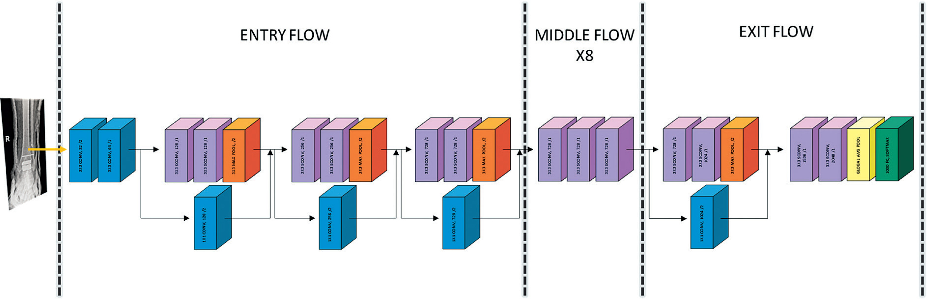
Figure 3
A) Confusion matrix for the training (left) and validation (right) set. B) Confusion matrix for the test set. The numbers in rectangles represent the count of predictions made by our model. The right-hand side gradient bar represents a visual scale of values equal to the number of instances in the rectangles. The scale differs for the training, validation, and test sets
Discussion
To the best of our knowledge, this is the first work that considers the use of AI to check the correctness of the AJ projection defined according to the recommendations of the literature. A paper concerning similar problems was published by Mairhöfer et al. [18]. The authors described the quality of the AJ radiographs, based on the subjective assessment of the radiologists, describing it on a scale from 1 to 3, where 1 means ‘perfect’ and 3 means ‘not diagnostic’. They use two networks: EfficientNet-B0 – twice, for radiographic view recognition and quality assessment, and DeepLabV3 – once, for region of interest extraction. In our project, we tested different classification networks including EfficientNet-B1 (upgraded version of EfficientNet-B0). This solution did not show promising results, while Xception was our network of choice.
We suggest that, excluding university medical institutions, the majority of radiology units possess hardware that is unable to provide sufficient power to process advanced multistep analysis of the submitted X-rays. Therefore, in contrast to Mairhöfer’s work [18], in our paper we present one-step analysis of the projection correctness, which could probably be performed in more diagnostic stations, even older ones, and in medical centres, without additional costs.
Another difference is that they do not discriminate between true AP and AP aimed at the DTFS and present the latter as a standard. Although there may be differences between countries, if it comes to a certain ‘standard’, we argue that each of those projections serves a different function, but the literature recommendations define the true AP projection as X-ray obtained with feet pointing forward, where the medial malleolus is not overlapping and the DTFS is not pointing towards an X-ray tube [12]. In practice, different radiology units may use slightly modified methods of quality assessment, whereas in our opinion, the literature guidelines should be applied similarly everywhere.
The advantage of our project compared to the one discussed is the three-step procedure. The model was evaluated in three stages, in which training was followed by validation and test, instead of performing two steps only (training and test). The validation procedure plays different roles, but the most important is to prevent overfitting; one could state that a result of above 90% in the setting of the authors test-set accuracy might be due to overfitting in the scenario of absence of a validation procedure.
However, our research appears to be complementary. Evaluating the accuracy of the projection axis and, subsequently, its quality, could provide a significant advantage to radiologists when compared to either of these aspects alone.
Two other papers related to the assessment of the quality of ankle X-ray images in the literature are conducted by Krönke et al. [19] and Köpnick et al. [20].
In Krönke’s study [19], the team uses the combination of two neural networks that provide spatial information about the AJ setting. With the use of a three-dimensional model generated from MRI images with different foot angular configurations, the second network acquires spatial information about bone contours. These markers are supplied by the first network, which identifies them in X-ray images, enabling the second network to compute the pertinent parameters for AJ orientation. The effects of the model’s operation are tested using an artificial foot model with real human bones at specific angulation settings.
In contrast to our experiments, which are based on determining the correctness of projection orientation and therefore answering the question of whether the projection was done according to the state of the art, this study focuses mainly on providing parameters for AJ positioning. Based on this, the user receives information about the angle of AJ position in relation to the detector, without a clear and straightforward determination of whether the taken image is correct or not, which is essential for further work with the radiograph.
Köpnick et al. [20] conducted a study similar to that of Mairhöfer [18], except that the data after training were compared to those obtained with a rotating phantom with known angular position for validation, and only one (the LAT projection) was used for testing. The similarity was the semi-subjective assessment of the visibility of the AJ articular space (divided into four classes, as opposed to Mairhöfer’s three). Contrary to what was presented by Mairhöfer and Köpnick, we believe that to assess the overall quality of a given projection, it is necessary to analyse the presence of other anatomical structures on the image to determine whether a given projection can be assessed as correct.
The main difference between the above-mentioned experiments and ours is that we took the approach that the X-ray would be assessed as is, refraining from the ROI definition. The specific projection of the AJ image according to the literature, as previously written, should include the relevant bony structures; hence, our correctness approach included the entire X-ray of the AJ.
Moreover, in our work we used X-rays of both healthy individuals and patients with various pathological conditions such as fractures, degenerative changes, and internal and external stabilisation (i.e. plaster cast). None of the aforementioned papers states the profile of the patient whose X-rays were used for the experiments, and this is of great importance because physicians are the ultimate recipients of the model’s results. It is likely that once the patient profile was standardised, our model would yield better results. In future work, we believe that for more complex images, such as those with advanced degenerative changes, the use of ROI or the notification to the physician of the need for manual evaluation would be required. An 89% accuracy with approximately 1100 non-standardised images is, in our opinion, a very good result.
Although there are papers concerning the role of AI in recognition of projection [21], we still lack research assessing the appropriation of each projection. Standardised, properly planned and performed X-ray imaging, especially in AJ, plays a crucial role in reliable analysis of a wide range of pathologies. It is hard to believe, but even some basic projections (i.e. AP versus AP mortise) are sometimes hard to distinguish from each other.
Conclusions
Given the similarities between commonly used projections, our model achieved high accuracy in recognising their correctness compared to an expert. The practical application of such a tool can also reduce the risk of under- or overdiagnosis, ultimately leading to medical error. This will directly result in reduced treatment costs and increased access to specialised care, as AJ problems are an increasing problem and are closely related to quality of life [22-24]. Machine learning tools approved by the FDA and recognised by the American College of Radiology are already being used in medicine [25].
Determining the correctness of the AJ projection is the first step in planning AJ arthroplasty. This procedure requires appropriate geometric measurements on radiographs. To make these measurements, it is necessary to devote a lot of specialists’ time to the evaluation of the examinations. Standardisation and proper evaluation of the correctness of the most commonly used AJ projections will make this procedure more accessible to patients.