

Introduction
The diagnosis of early-stage breast cancer relies on a combination of clinical assessments, radiological imaging, and biopsy confirmation. Magnetic resonance imaging (MRI) is one of the commonly used tools in the screening, problem-solving, and tumor staging of breast cancer. One specialized technique, diffusion-weighted imaging (DWI) with apparent diffusion coefficient (ADC) mapping, offers detailed insights into the various compartments within tissue, and this has been found to improve diagnostic accuracy. This technique is frequently used in multiparametric imaging setting to detect and characterize breast tumors [1-3]. Dynamic contrast-enhanced MRI (DCE-MRI) is another diagnostic technique that is used to depict breast lesions, relying upon both morphologic and hemodynamic features [4]. However, there are instances where benign breast lesions may display strong contrast enhancement similar to malignant lesions, which can lead to a false positive diagnosis, unnecessary biopsies or overtreatment [5].
Breast cancer is a heterogeneous tumor characterized by a diverse tumor microenvironment. Recent studies indicated that increased intra-tumor heterogeneity is associated with unfavorable clinical outcomes [6,7]. Therefore, understanding the spatial heterogeneity of a tumor is crucial for making effective treatment decisions [8,9]. Non-invasive imaging techniques that can fully exploit this intratumor heterogeneity are highly valued in the diagnosis, tumor staging, and assessment of therapy response [10]. Tumor habitat analysis is one such technique that can identify distinct cell populations and tumor subregions via mathematical modeling and quantitative imaging. Specifically, each habitat represents subregions containing clusters of voxels with similar features [8,11]. Habitat imaging combines multiparametric MRI to determine the quantitative imaging characteristics of tumors, providing insight into the spatial distribution of tumor subregions [12].
The fractal dimension (FD) is a scale-invariant parameter to characterize complex and non-regular objects. It represents the morphological complexity and self-similarity of objects as measured on different scales. The estimation of FD using fractal analysis has shown great potential in several clinical applications such as grading meningioma, central nervous system lymphoma, glioblastomas, and grading of intervertebral disk degeneration [13-16]. However, this approach has primarily focused on the entire lesion, without considering the internal structural complexity.
By using advanced mathematical modeling, habitat imaging can divide tumors into distinct subregions, allowing for the spatial tumor habitat clustering of voxels with similar radiomics features [17]. In this study, we aimed to assess the intratumoral heterogeneity by combining DWI and DCE-MRI data, and by calculating the box-counting FD of each habitat. Herein, we introduced a novel approach that used fractal analysis to examine the complexity of tumor subregions, showing improved diagnostic performance in differentiating malignant and benign lesions compared to analyzing the heterogeneity of the whole lesion using the FD as a classifier.
Material and methods
Subjects
From our electronic hospital information system, we retrospectively identified 107 patients with 112 breast lesions including 78 malignant lesions (median age, 58 years) and 34 benign lesions (median age, 48 years) who were treated between January 2019 and June 2023 and met the following inclusion criteria: 1) histopathologically verified benign lesions or breast cancer; 2) underwent conventional breast MRI examinations, including DWI and 5-phase DCE-MRI; 3) had a measurable contrast-enhancing lesion and a detectable lesion on DWI with largest lesion diameter ≥ 1 cm; and 4) adequate imaging quality. To avoid mismatching with histopathological results, the inclusion criteria in the diagnostic performance analysis was that no treatment occurred between biopsy and imaging. The median interval between preoperative MRI examinations and definitive breast biopsy or surgery was 6 days (range, 2-21 days). A total of 75 malignant lesions and 32 benign lesions were evaluated, as some patients had multiple lesions, and the lesion with the largest size was included. Detailed patient and lesion information is shown in Table 1. The study was approved by the local institutional review board (No. 2023-193). As it was a retrospective study, the requirement for written informed consent was waived.
Table 1
Clinical and pathological characteristics of patients
| Variables | Benign lesions (n = 34) | Malignant lesions (n = 78) |
|---|---|---|
| No. of patients | 32 | 75 |
| Age (years) | 48.0 (40.0, 58.8) | 58.0 (46.0, 64.0)a |
| Lesion size (largest diameter) (mm) | 24.0 (16.8, 29.8) | 25.0 (20.0, 37.0) |
| Histopathology | 25 (73.5) fibroadenomas | 67 (85.9) invasive ductal carcinomas |
| 6 (17.6) intraductal papillomas | 4 (5.1) ductal carcinomas in situ | |
| 1 (2.9) adenosis | 4 (5.1) invasive lobular carcinomas | |
| 2 (5.9) other benign lesions | 3 (3.8) invasive micropapillary carcinomas |
Magnetic resonance image acquisition
The MRI studies were performed using a 3.0T MRI system (uMR 780, United Imaging Healthcare, Shanghai, China) with a dedicated phased-array breast coil. In all cases included, a standard protocol was performed, including: 1) bilateral axial non-contrast T1-weighted, 2) axial fat-suppressed T2-weighted, 3) pre-contrast axial DWI, and 4) axial dynamic contrast-enhanced pre-contrast and post-contrast fat-suppressed GRE_quick 3D T1-weighted imaging.
Spin-echo echo-planar imaging was used to generate DWI and corresponding ADC maps in the axial plane. The DWI parameters were as follows: repetition time (TR)/echo time (TE), 3702/67 ms; slice thickness = 4 mm, 24 slices; parallel imaging factor, 2; flip angle, 90°; matrix size, 192 × 192; field of view, 190 × 380 mm; b-values = 50, 600, 1000 s/mm2; and total imaging time, 3 min 2 s. The T1 GRE_quick 3D DCE-MRI sequence was acquired in the axial plane using the following parameters: TR/TE, 4.8/1.99 ms; slice thickness = 1 mm, 144 slices; echo train length, 20; pixel bandwidth, 450 Hz; compressed sensing (CS) acceleration factor, 5; flip angle, 10°; matrix size, 336 × 336; field of view, 340×340 mm. The total acquisition time was 7 min 34 s. The DCE-MRI series consisted of 6 frames: one pre-contrast and 5 post-contrast. After the pre-contrast images were acquired, the contrast agent, 0.1 mmol/kg gadopentetate dimeglumine (Shanghai Xudong Haipu Pharmaceutical Co., Ltd., Shanghai, China), was intravenously injected at a rate of 2 ml/s, followed by 20 ml of saline solution at the same rate.
Image reconstruction and data analysis
The image reconstruction and data analysis procedures in this study were based on methodologies established in previous work [18]. Spatial tumor habitats were analyzed using reconstructed ADC maps and perfusion maps, specifically the wash-in and wash-out maps. ADC maps were generated from DWI data acquired with three b-values using a mono-exponential diffusion model. For perfusion mapping, images from specific phases of DCE-MRI were used. The wash-in map was created by subtracting the pre-contrast image from the second-phase image, while the wash-out map was obtained by subtracting the fifth-phase image from the second-phase image.
As previously described [18], co-registration of ADC and DCE-MRI images was performed using affine transformations – including rigid body and scaling adjustments – implemented via the Advanced Normalization Tools software package. To prepare the data for clustering analysis, ADC maps were resampled to match the isotropic resolution of the DCE-MRI using B-spline interpolation. Histogram matching was applied to standardize MRI intensity distributions across all patients, minimizing variations due to different acquisition settings and facilitating consistent clustering.
The patient data were divided into training (70%) and testing (30%) cohorts. In the training cohort, intratumoral subregions – or habitats – were identified using k-means clustering applied to a three-dimensional parametric space constructed from the diffusion and perfusion features [19]. Clustering was performed at the cohort level to stabilize habitat assignments across patients and address inter-tumor heterogeneity. The optimal number of clusters (k = 3) was determined based on evaluation metrics such as the Calinski-Harabasz score and Silhouette coefficient, aiming for a balance between model simplicity and data interpretability [7,20]. Intratumoral heterogeneity was quantified by calculating, for each voxel, the proportion of its eight neighboring voxels that belonged to different habitats, then averaging these values across the entire tumor volume. This method captures the local variability within the tumor microenvironment.
The FD of each habitat’s edge was calculated to assess the complexity and roughness of tumor boundaries. The box-counting method was employed, as detailed in previous studies [14,15]. This method involves covering the tumor edge with non-overlapping boxes (or voxels) of varying sizes and counting the number of boxes N_α required at each scale α.
The FD is mathematically defined as:
In practice, the FD was estimated by plotting log(N(α)) against log(1/α) and calculating the slope of the linear portion of this plot. A set of scale ratios was used to vary α: 2, 3, 4, 5, 6, 7, 8, 9, 10, 20, and 50. Each ratio corresponds to analyzing the image at different resolutions; for instance, a ratio of 2 means each box covers 2 × 2 × 2 original voxels.
As the scale increases (larger α), the number of boxes N_α required to cover the fractal structure decreases, approaching one at very large scales. This relationship can lead to saturation in the curve at high scales, emphasizing the importance of selecting an appropriate range for α. By using multiple scales, the FD calculation captures how the complexity of the tumor edge changes with resolution. A higher FD indicates a more intricate and irregular edge morphology (Supplementary Material Figure S1), reflecting increased roughness and potential heterogeneity at the tumor boundary. This metric provides insight into the structural complexity of the tumor habitats, which may correlate with underlying biological processes. For each lesion included in this study, the tumor volume of interest was determined by manual slice-by-slice segmentation on DCE-MRI images without including peritumoral tissues. The corresponding data were stored in the Neuroimaging Informatics Technology Initiative format. Lesion segmentation was independently performed by two radiologists with more than 6 years of experience in breast MRI.
Statistical analysis
Descriptive statistics presented are mean ± standard deviation, median (interquartile range [IQR]) for continuous variables, or n (%) for categorical variables. The Shapiro-Wilk test was used to evaluate the normality of all continuous variables. Inter-reader variability in 3D region of interest (ROI) definition was measured using the Dice similarity coefficient, and the inter-reader reliability for FD was performed using the intraclass correlation coefficients. Median FD values of malignant and benign groups were compared using the Mann-Whitney U test. ROC curve analysis was performed to determine the optimal FD cut-off value in order to differentiate benign from malignant lesions. The sensitivity, specificity, and area under curve (AUC) for the ROC analysis were calculated. All statistical analyses were conducted using standard software, including GraphPad Prism v8.0 (GraphPad Software, Inc. San Diego, CA, USA) and MedCalc v.20 (Ostend, Belgium). A p-value < 0.05 was considered statistically significant.
Results
Clinical and pathological characteristics
The detailed clinical, pathological, and imaging characteristics of the two groups of patients are summarized in Table 1. The median age of the malignant group (58) was significantly higher than that of the patients with benign lesions (48, p = 0.032). There was no significant difference in lesion size (largest diameter) between the two groups (p = 0.254).
Inter-reader reliability of 3D ROI definition and FD
The overall Dice similarity coefficient across all lesion classes was 0.86 (95% confidence interval [CI]: 0.79-0.96). The inter-reader reliability was excellent, with intraclass correlation coefficients of 0.95 (95% CI: 0.92-0.99) for the average local heterogeneity of the entire lesion, 0.96 (95% CI: 0.94-0.99) for hypervascular cellular FD, 0.92 (95% CI: 0.89-0.96) for hypovascular cellular FD, and 0.93 (95% CI: 0.90-0.97) for nonviable tissue FD.
MRI habitat characteristics of tumor subregions
The optimum number of clusters was determined to be three based on the averaged Calinski-Harabasz score and Silhouette coefficient (Supplementary Material Figure S2). Three habitats were defined as a hypervascular cellular habitat (high wash-in and high wash-out), a hypovascular cellular habitat (low ADC and low wash-in/wash-out), and a nonviable tissue habitat (high ADC and low wash-in/wash-out). Statistically significant differences in the volume fraction of the hypervascular cellular habitat (p < 0.001) and nonviable tissue habitat (p < 0.001) between the malignant and benign lesions were observed. There were no statistically significant differences in the hypovascular cellular habitat (p = 0.314) between the malignant and benign lesions (Supplementary Material Figure S3).
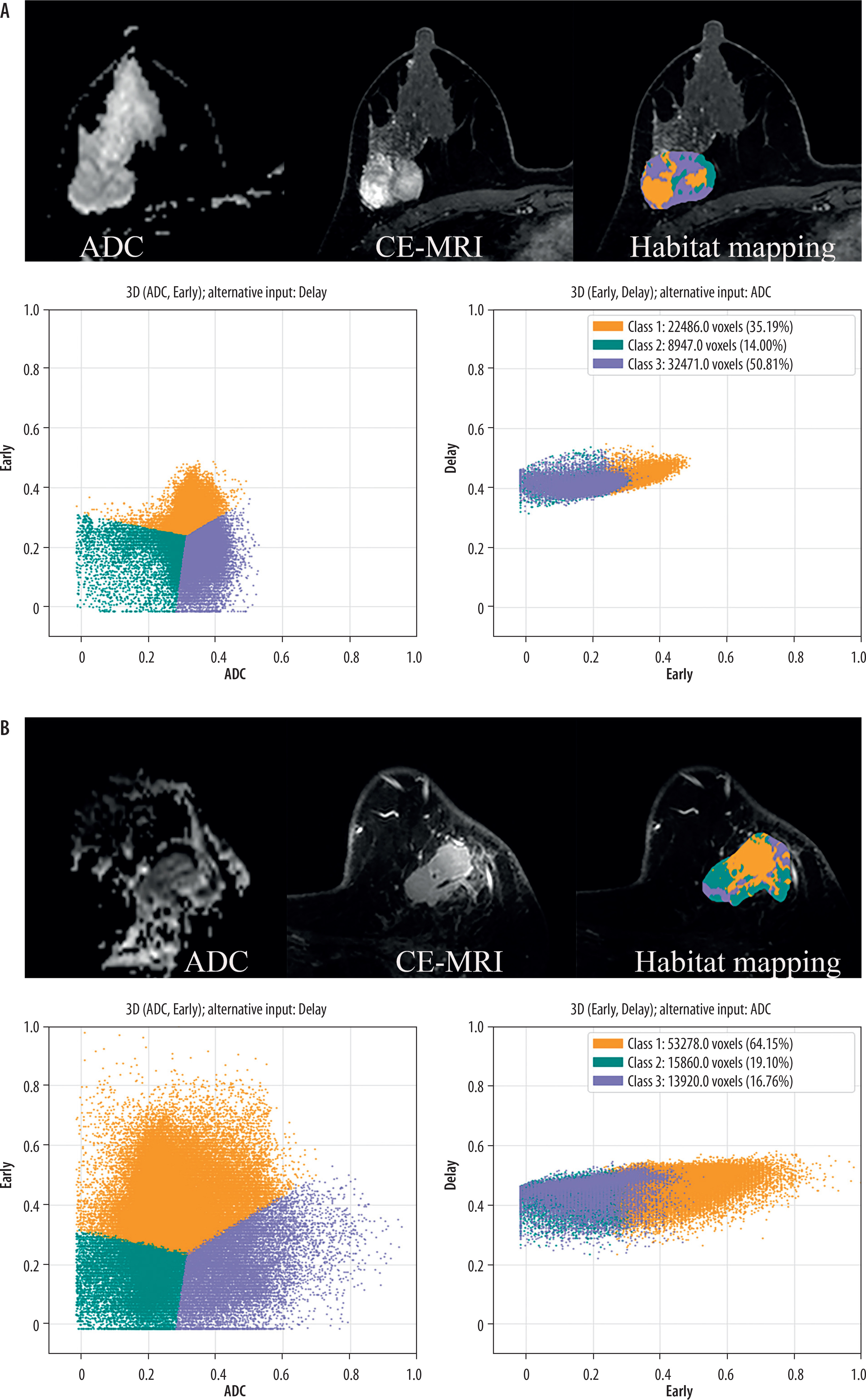
Accordingly, three physiological FDs were defined as hypervascular cellular FD, hypovascular cellular FD, and nonviable tissue FD, corresponding to the above-mentioned three habitats. The average hypervascular cellular FD was found to be statistically significantly different (p < 0.001) between malignant and benign lesions (Figure 1). The median hypovascular cellular FD of the malignant group (0.84, IQR: 0.82-0.87) was significantly higher (p < 0.001) than that of the patients with benign lesions (0.56, IQR: 0.37-0.78). A statistically significant difference was absent in nonviable tissue FD (p = 0.568). A statistically significant difference between malignant and benign lesions was found for the conventional heterogeneity of the whole lesion (p = 0.015). Figure 2 illustrates example maps of tumor habitats for malignant and benign lesions.
Figure 1
Box plots of the heterogeneity of the whole lesion and fractal dimension (FD) of each habitat between the malignant and benign lesions. A statistically significant difference between malignant and benign lesions was found for the heterogeneity of the whole lesion (A), hypervascular cellular FD (B) and hypovascular cellular FD (C). No statistically significant difference was found in the nonviable tissue FD (D)
The lines in the boxes indicate medians, and the boundaries of the boxes indicate the lower and upper quartiles. p < 0.05
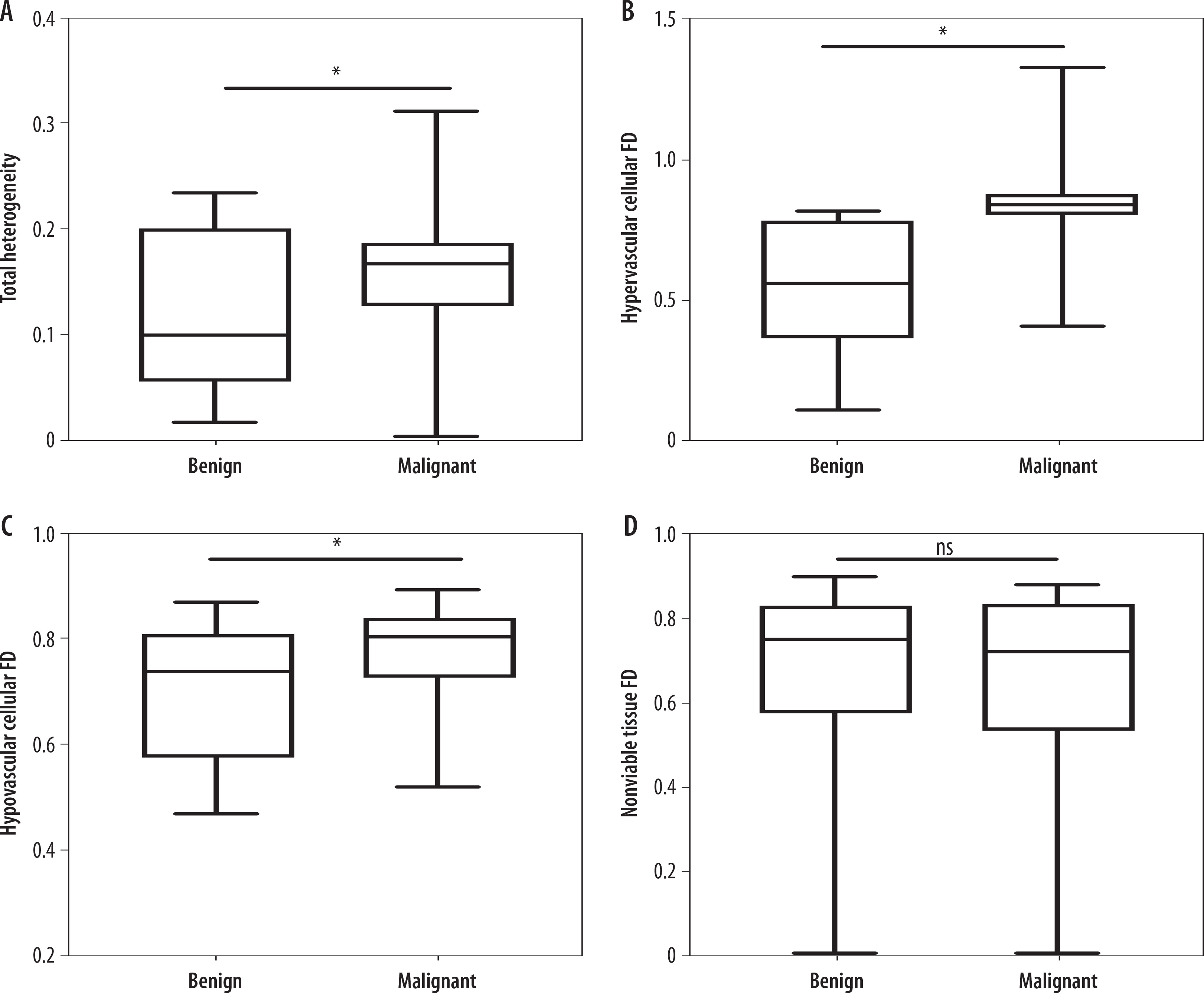
Figure 2
Two examples of tumor habitats on magnetic resonance imaging (MRI): A) A patient with a benign fibroadenoma showing a smooth boundary. Most of the lesion was occupied by the nonviable tissue habitat (purple); B) A patient with invasive ductal carcinoma showing irregular shape and spiculated margin. Most of the lesion showed predominance of the high vascularity and cellularity habitat (yellow), contributing to continued tumor growth
To construct physiological tumor habitats, k-means clustering was applied to the apparent diffusion coefficient (ADC) (3 b-values diffusion-weighted imaging) and perfusion parametric maps (the pre-contrast, the second and the fifth phase images of the dynamic contrast-enhanced MRI). Representative parameter maps and corresponding habitat maps are shown in the bottom row of Figure 2A and 2B. The hypervascular cellular habitat with high vascularity and cellularity (yellow), hypovascular cellular habitat with relatively low wash-in map and relatively low ADC (green), and nonviable tissue habitat with relatively high ADC and relatively low wash-in map (purple) all show distinct differences in their values
Diagnostic performance of three physiologic MRI habitat-based FD
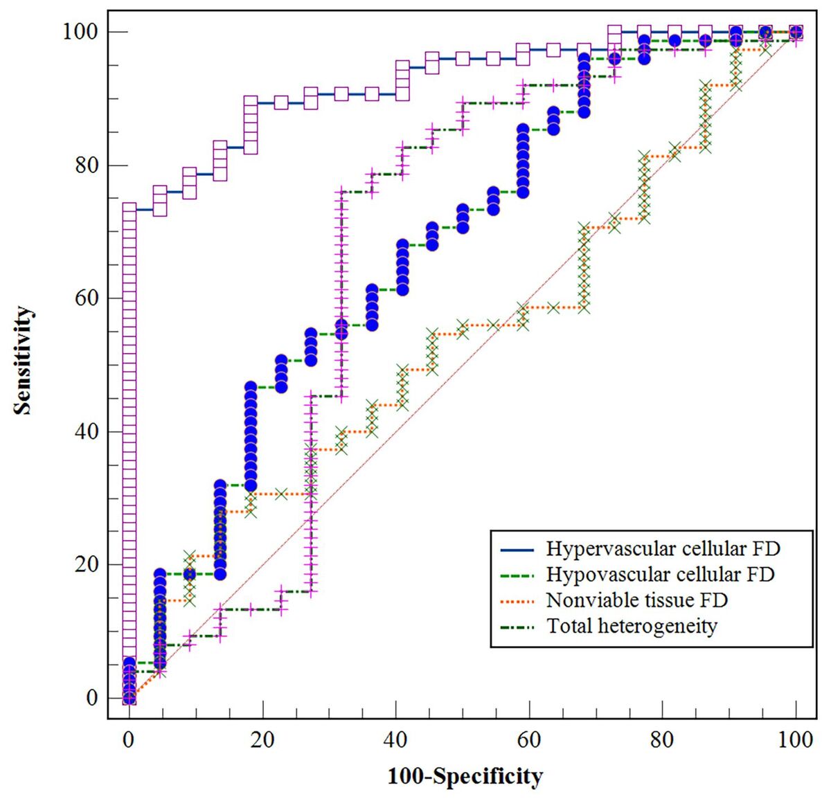
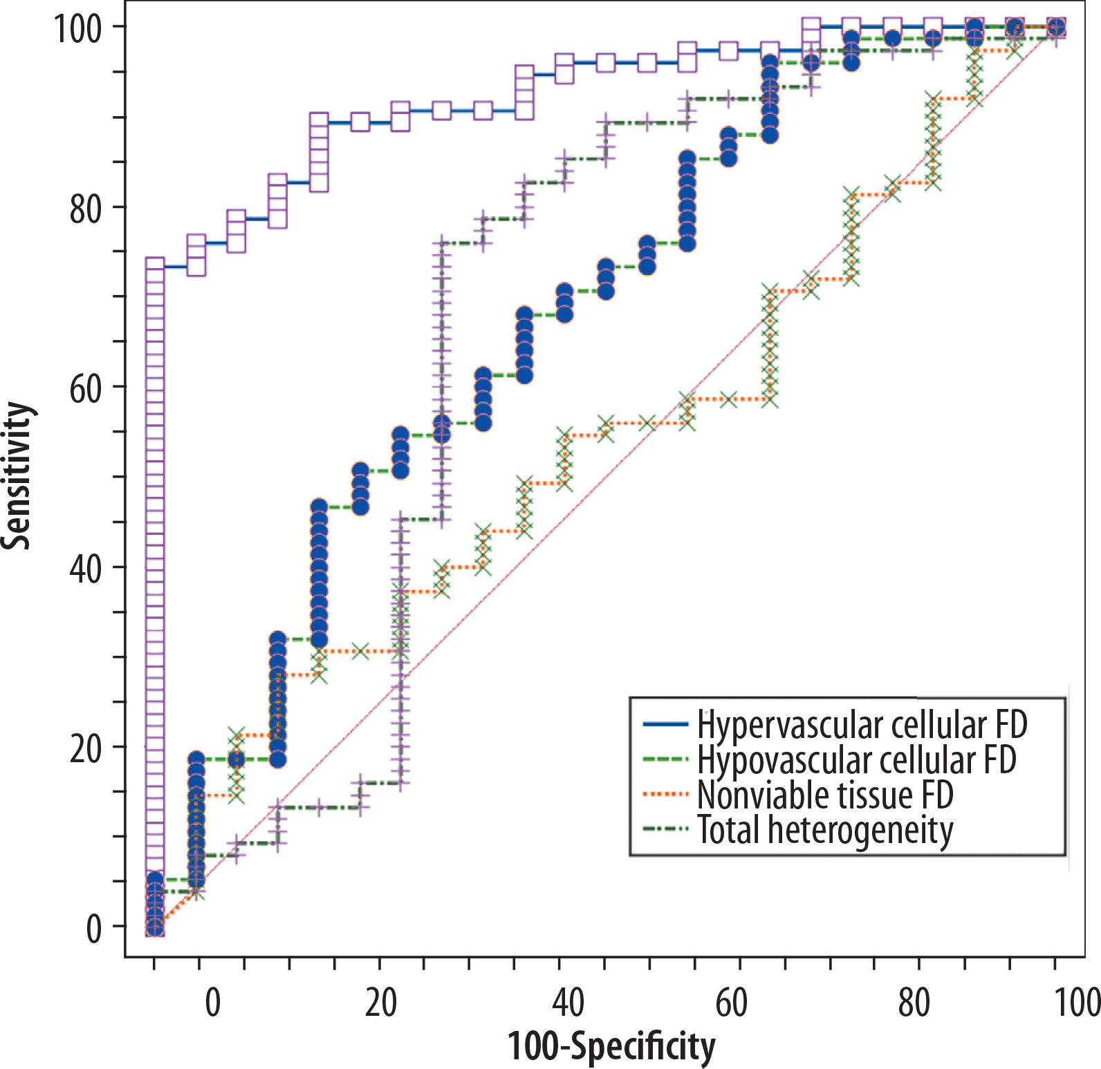
The diagnostic accuracies of the estimated FD and the heterogeneity of the whole lesion to differentiate malignant lesions from benign cases were compared in terms of the AUC, as shown in Figure 3 and Table 2. The AUC of the hypervascular cellular FD (0.925, 95% CI: 0.854-0.969) was the highest among the fractal analysis parameters and higher than that of the total heterogeneity of the whole lesion (0.671, 95% CI: 0.568-0.763). Additionally, the AUC of the hypervascular cellular FD was higher than those of the volume fraction of the three physiologic MRI habitats (hypervascular habitat: 0.744, 95% CI: 0.646-0.827; hypovascular cellular habitat: 0.572, 95% CI: 0.467-0.672; nonviable tissue habitat: 0.767, 95% CI: 0.670-0.847 (Supplementary Material Figure S4 and Table S1).
Table 2
Diagnostic characteristics of subregional fractal dimension (FD) features and total heterogeneity to classify malignant lesions from non-malignant lesions
| Variables | Cut-off value | AUC (95% CI) | Sensitivity (95% CI) | Specificity (95% CI) | PPV (95% CI) | NPV (95% CI) |
|---|---|---|---|---|---|---|
| Hypervascular cellular FD | 0.784 | 0.925 (0.854-0.969) | 89.3 (80.1-95.3) | 81.8 (59.7-94.8) | 94.4 (87.3-97.6) | 69.2 (53.2-81.7) |
| Hypovascular cellular FD | 0.808 | 0.679 (0.576-0.770)a | 46.7 (35.1-58.6) | 81.8 (59.7-94.8) | 89.7 (77.7-95.6) | 31.0 (25.2-37.5) |
| Nonviable tissue FD | 0.542 | 0.535 (0.431-0.637)a | 28.0 (18.2-39.6) | 86.4 (65.1-97.1) | 87.5 (69.7-95.5) | 26.0 (22.1-30.4) |
| Total heterogeneity | 0.127 | 0.671 (0.568-0.763)a | 76.0 (64.7-85.1) | 68.2 (45.1-86.1) | 89.1 (81.3-93.8) | 45.5 (33.7-57.7) |
Figure 3
The receiver-operating characteristic curve (ROC) for the heterogeneity of the whole lesion and fractal dimension of each habitat in differentiating malignant and benign lesions
Area under the ROC for hypervascular cellular fractal dimension (FD), hypovascular cellular FD, nonviable tissue FD, and total heterogeneity was 0.924, 0.708, 0.536, and 0.671 respectively, to identify malignant from benign lesions according to the DeLong test
Discussion
Tumor heterogeneity presents a major challenge in making treatment decisions. Current approaches, such as histogram and texture analysis, only assess spatial variations throughout the entire tumor and assume that the tumor is a uniform entity. In contrast, habitat imaging can identify distinct tumor subregions that reflect different functional or material areas of focus. Previous studies have used habitat imaging with multiparametric quantitative MRI to detect intratumoral heterogeneity in glioblastoma, brain metastases, and breast cancer [8,20,21].
Imaging biomarkers that stratify patients with clinical relevance are crucial for precision medicine. Fractal analysis measures the complexity of a structure or image, such as computed tomography or MRI, with a higher value indicating increased object complexity [22]. Fractal analysis is a promising tool for evaluating texture characteristics on MRI, offering stability and reduced susceptibility to imaging noise compared to other texture features [14,15]. To our knowledge, there is no predictive model that combines tumor habitat MRI and fractal analysis to characterize intratumoral heterogeneity. This method plays an important role in supporting the diagnosis, monitoring, and treatment of breast cancer. In this study, we calculated the FD of each habitat to address this issue.
Differentiating between benign and malignant breast lesions before treatment has significant clinical implications. This study investigated the feasibility of FD in habitat analysis with tumor subregion complexity for the differential diagnosis of benign and malignant breast lesions. Beyond the volume fraction of each habitat, the spatial distribution of the habitats showed significant diagnostic power. The FD in this study reflected the complexity of each habitat based on heterogeneity, demonstrating that the complexity of the hypervascular habitat in malignant breast lesions was greater than that in benign lesions. Given the correlation between heterogeneity and invasiveness [23], this phenomenon corresponded to the breast cancer being more invasive [24].
Malignant breast lesions exhibited significantly higher heterogeneity than benign lesions, suggesting that breast cancer presents a more complex heterogeneity pattern on MRI. Previous studies have shown that aggressive breast cancers, especially the triple-negative subtype, contain necrosis, which may exhibit a highly heterogeneous distribution of proliferating cells within the tumor, leading to irregular shapes [25,26].
The key finding of this study is that the hypervascular cellular FD significantly improved the diagnostic performance compared to the traditional heterogeneity of the whole lesion. The AUC increased from 0.671 to 0.925, indicating that heterogeneity with tumor subregion complexity independently represents tumor aggression. This may explain the inconsistency of previous studies where only the volume fraction was compared [27,28]. Hypervascular cellular FD has the potential to become a powerful and useful imaging biomarker.
Our results indicate that the hypervascular cellular habitat with relatively low ADC and wash-in map (early phase) has a remarkable ability to discriminate breast cancer from benign lesions. The hypervascular cellular habitat represents a subregion with high vascularity and cellularity, which likely corresponds to the aggressive component of the tumor. Angiogenesis is a hallmark of breast cancer, and the new capillaries within the tumor are immature, tortuous, and hyperpermeable, leading to spatial heterogeneity [29,30]. Prior studies have demonstrated that breast cancer molecular subtype is associated with vascular features [31]. With DCE-MRI, highly vascularized tumors tend to exhibit strong contrast enhancement in the early phase and wash-out of contrast in the delayed phase. Our data provide further evidence of the correlations between the percentage tumor volume of high-cellularity or high-vascularity habitat and histological measures of macrophage infiltration or vascularity in pathological studies [8,32].
One of the challenges highlighted in this study is the classification of lesions or voxels with high wash-in and low wash-out characteristics, which is not directly accounted for in the three defined habitats. This challenge emphasizes the complexities of the parametric space and the interpretability of clusters. The choice of k = 3 was grounded in the desire to circumvent overparameterized models and maintain a level of simplicity in data interpretation. With this in mind, the clusters, while aiding in general understanding, may not strictly correspond to descriptive labels such as “hypervascular cellular,” “hypovascular cellular,” and “nonviable tissue” for every single tumor, considering the inherent variability in tumor characteristics. While the k-means clustering algorithm assigns each voxel based on its proximity to centroids, a voxel exhibiting high wash-in and low wash-out rates does not neatly fit into our predefined habitats. The absence of a distinct cluster for such voxels might be seen as a limitation. However, it also emphasizes the continuous spectrum of biological behaviors that exists within individual tumors and across different tumors. In practice, the tumor habitats rarely present as well-defined entities. The current model’s simplifying assumption does allow for meaningful interpretation and aids in understanding the general patterns of tumor biology. Refining the clustering strategy to account for a broader range of parametric features, such as incorporating more clusters or utilizing more advanced clustering techniques, could potentially improve the model’s accuracy and the granularity of results. Future studies could consider these enhancements to better account for the diversity of vascular behaviors in tumors, ultimately providing a more comprehensive picture of tumor heterogeneity.
At the same time, this study has several limitations. Firstly, its retrospective nature lacks precise pathological confirmation of the image-based segmentation. Therefore, labeling clusters as “hypervascular habitat,” “hypovascular cellular habitat,” or “nonviable habitat” raises the potential for discrepancies between imaging classifications and their corresponding pathological states. This potential inconsistency underscores the concern about inter-tumor heterogeneity and the potential mislabeling based on the selected clusters. Secondly, the analyzed dataset was collected from a single center, limiting the generalizability and applicability of the proposed model. Thirdly, only the largest lesion was considered in several patients with multifocal breast lesions. Finally, it remains unclear whether the three spatial habitats displayed similar patterns in breast lesions with a diameter less than 10 mm compared to those with a diameter greater than or equal to 10 mm. Further studies are needed to clarify the minimum size of a breast lesion required for the FD features generated by habitat imaging.
In conclusion, this pilot study reveals that the FD features generated by habitat analysis can better differentiate benign from malignant breast lesions compared to the total heterogeneity features extracted from the whole tumor. The predictive model combining tumor habitat MRI and fractal analysis could prove useful as a screening tool. Our data suggest that fractal analysis may play an essential role in identifying patients whose breast lesions are more likely to behave aggressively.