Introduction
The liver is the largest gland in the human body and plays a vital role in metabolic regulation, detoxification, immune modulation, and nutrient storage [1]. Chronic liver disease (CLD) refers to the progressive deterioration of hepatic function over at least six months, involving ongoing inflammation, fibrosis, and regenerative changes that may culminate in cirrhosis [2]. A wide range of etiological factors such as chronic alcohol use, viral hepatitis, autoimmune liver disorders, and genetic metabolic syndromes contribute to the development of CLD. Cirrhosis, the end stage of CLD, leads to structural distortion of the liver, vascular remodeling, and extracellular matrix accumulation, which ultimately impairs hepatic function and increases the risk of complications [2]. CLD remains a major global health burden, especially in resource-limited settings, with increasing prevalence reported in recent epidemiological studies [3].
Accurate diagnosis of CLD often requires radiologic imaging in addition to clinical and laboratory data. While ultrasound is a common first-line modality, magnetic resonance imaging (MRI) is preferred in many cases due to its high soft tissue contrast and radiation-free nature [4,5]. MRI allows for detailed anatomical and tissue characterization and has become a cornerstone in liver imaging.
In recent years, artificial intelligence (AI), particularly deep learning (DL), has shown promise in enhancing image interpretation and disease classification in radiology. Many previous studies have employed DL models using computed tomography (CT) images or histopathological data [6-16]; however, studies using MRI data especially without manual segmentation remain limited [17,18]. One of the distinguishing features of this study is the use of raw MRI images without any segmentation process. Instead of manually isolating liver regions or lesions, we propose a model that directly processes axial and coronal MRI sequences, aiming to increase practicality, reduce preprocessing time, and maintain reproducibility across datasets.
In this context, the objective of our study was to develop a deep convolutional neural network (DeepCNN) model that can classify CLD versus non-CLD cases directly from non-segmented MRI images. By incorporating multiple MRI sequences and viewing planes, this approach seeks to reflect real world variability and clinical applicability, while also contributing to the relatively underexplored area of MRI-based DL for liver disease detection.
Material and methods
This retrospective study was approved by Eskişehir Osmangazi University Non-Interventional Clinical Studies Ethics Committee (date: 27.02.2024, decision No. 53). A DeepCNN model was developed to detect CLD using MRI data. The dataset is composed of patient data collected between January 2018 and January 2024. Various techniques were employed to optimize model performance and adaptively improve the learning process.
Dataset/pre-processing
The dataset used in the study contains 184 patients in total. The dataset includes images of different sequences (axial T1 without lava contrast, axial T2 without fat suppression, coronal T2 without fat suppression) in both axial and coronal planes. The dataset consists of 1112 images, of which 460 are normal and 652 are chronic liver MRI images. The images in the dataset were obtained from dynamic liver MRI examinations performed by a 3-Tesla (General Electric, Milwaukee, Wisconsin) MRI machine.
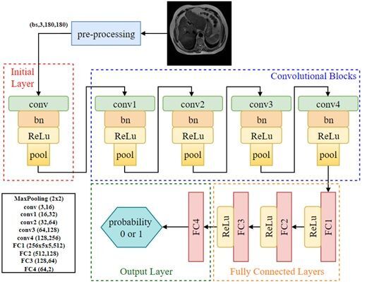
The dataset consisted of 1112 MRI slices from 184 patients, including both axial and coronal views. Specifically, 722 axial and 390 coronal images were included, and both imaging planes contained samples from normal and CLD classes. Images were input individually into the model, regardless of their orientation. No fusion method or explicit indication of image plane was used during training. This approach was chosen to evaluate the model’s ability to generalize across imaging planes and to reflect real-world variability in radiology practice. Examples of the dataset used are shown in Figure 1.
Figure 1
Coronal and axial images of normal/chronic liver disease (CLD) patients from the data set used
In order to enhance the model’s generalization capability and mitigate overfitting, data augmentation techniques were applied dynamically during the training phase. First, all images were resized to 224224 pixels to ensure consistent input dimensions for the model and to train it with fixed size inputs. To apply data augmentation, the images were randomly flipped horizontally with a 50% probability, enabling the model to generalize better to horizontally symmetric data and reduce overfitting. Additionally, the images were randomly rotated between –10 and +10 degrees to make the model more robust to rotational variations. This, too, served as a form of data augmentation. The brightness, contrast, saturation, and hue of the images were randomly adjusted in small proportions to increase the model’s generalizability to different lighting conditions and color variations. The images were then cropped to 180 180 pixels from the center, a step aimed at reducing noise at the image edges and focusing on the cetral region, which is often more important for the model to learn relevant features. Lastly, the images were converted into tensors for use in PyTorch.The tensor transformation normalized the pixel values to a range of (0,1), preparing the images in a format suitable for the model’s input. In the final step of preprocessing, additional data augmentationtechniques, such as rotation, translation, scaling,and brightness adjustments, were applied to further increase the diversity of the training dataset. These transformations were implemented in real time, meaning that they did not increase the nominal size of the dataset, which remained at 1112 images. However, they effectively expanded the diversity of the training data by generating different representations of the same images across epochs.
Model architecture
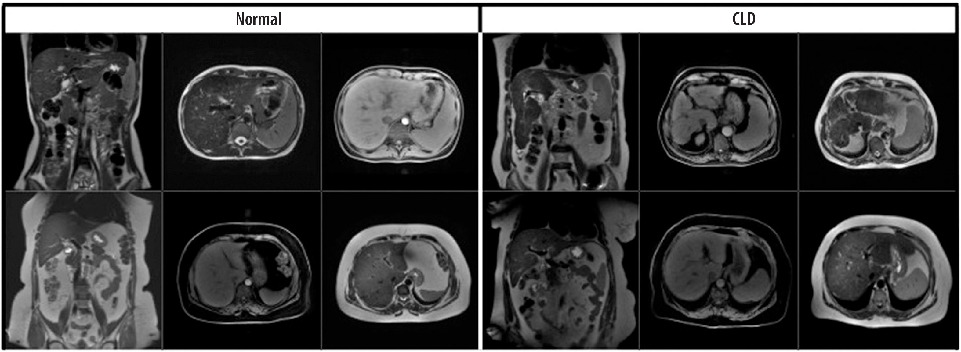
The fundamental architecture of the model is based on a DeepCNN and is designed for a binary image classification task. The architecture begins with a convolutional layer that processes input images and extracts basic features, followed by multiple convolutional layers that progressively extract both low- and high-level features. These convolutional layers are interspersed with max pooling layers, which reduce the computational complexity by downsampling the feature maps. In the model architecture, batch normalization (BN) layers are used after each convolutional layer to stabilize and accelerate the training process by normalizing the input distributions. Batch size (BS), on the other hand, refers to the number of samples processed together in a single forward and backward pass during training. A BS of 16 was used in this study to balance learning efficiency and computational cost. The features extracted by the model are then fed into fully connected layers to produce the final class predictions. Lastly, the output layer provides a probability distribution across the chronic and normal classes (0 or 1), facilitating the final classification decision.
The developed DeepCNN model, whose architecture is illustrated in Figure 2, is structured as follows:
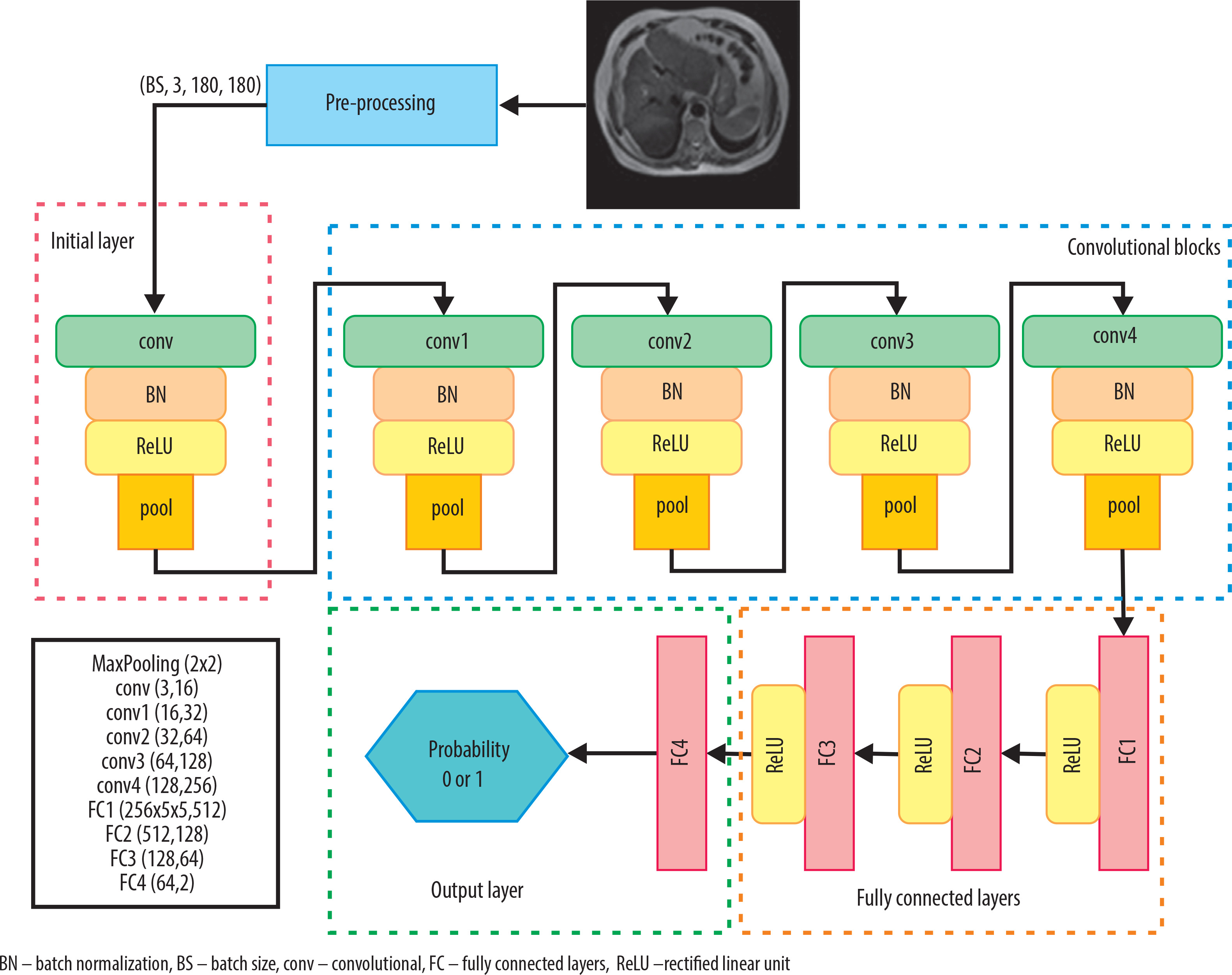
Initial layer: The input image, consisting of 3 channels (RGB), is processed with a 33 convolution filter to extract 16 feature maps. This layer is followed by BN (with 16 channels) and a rectified linear unit (ReLU) activation function, and then max pooling with a 22 filter.
Convolutional blocks: In the second stage, the input images pass through four convolutional layers with 32, 64, 128, and 256 filters, respectively. Each convolutional layer is followed by BN and activated using the ReLU function. A 22 max pooling operation is applied between layers to reduce the spatial dimensions. These layers are designed to progressively learn higher level features of the images.
Fully connected layers: The feature maps obtained from the convolutional layers are flattened and fed into three fully connected layers. The first fully connected layer maps the 25655 input vector to 512 units. The output is then passed through two additional fully connected layers with 128 and 64 units, respectively, each using the ReLU activation function.
Output layer: The final fully connected layer with 64 units is followed by a fully connected layer with 2 output units for classification. The FC4 layer produces logits scores for the two classes. This represents the class probabilities predicted by the model. The torch.max function determines the predicted class by selecting the highest logits score. The class is indexed by the highest scoring tensor value: if the index is 1, the class is labeled “Chronic Liver”; if 0, the class is labeled “Normal.”
Training and optimization
The Cross-Entropy Loss function was used to train the model. The Adam optimization algorithm was selected for optimization, with an initial learning rate of 0.0001. To enhance the model’s performance, the learning rate was halved every 5 epochs using learning rate scheduler. During the training process, the best model weights were preserved based on the highest accuracy and lowest validation loss. Additionally, the learning rate was increased by 10% when the validation accuracy improved, and decreased by 10% when the validation loss was reduced. A cross-entropy loss function was employed to minimize classification errors during training. To accelerate training and make it more efficient, Adam was chosen as the optimizer, as it uses adaptive learning rate methods to maintain a stable learning process. At different stages of training, the model’s learning rate was dynamically adjusted to ensure both fast and stable learning. Furthermore, the model’s performance was continuously monitored on the validation dataset, and early stopping criteria were applied to prevent overfitting.
Model evaluation
The performance of the model was evaluated with metrics such as accuracy, precision, recall, and F1-score.
Accuracy: The correct prediction rate of the model was calculated.
Precision: Measures how much of the images classified as chronic are actually chronic. High precision indicates that the model has a low false positive rate.
Recall: Measures how much of the truly chronic images are correctly classified. High sensitivity indicates that the model has a low false negative rate.
F1-score: Calculated as the harmonic mean of sensitivity and recall.
Test accuracy: The ratio of correctly classified samples to total test samples in the test dataset.
Confusion matrix (CM): True positive (TP): correctly predicted instances for Class 1. True negative (TN): correctly predicted instances for class 0. False positive (FP): instances incorrectly predicted as class 1 when they were class 0. False negative (FN): instances incorrectly predicted as class 0 when they were class 1.
Disease prediction using machine learning algorithms
Traditional machine learning (ML) algorithms are widely used for disease diagnosis and detection. Classification algorithms such as logistic regression, k-nearest neighbor (KNN), support vector machines (SVM), and random forest have been effectively employed in disease diagnosis [19-22]. To compare with our developed DeepCNN model, we applied logistic regression, KNN, SVM, and random forest methods using our database.
Training the model
During the training process, the dataset was divided into training, validation, and test sets. Initially, all patient images were categorized into two main groups: normal and CLD. These patient-level groups were then randomly split into training (87.3%), validation (5.0%), and test (7.7%) sets within the program. Images designated as test data were excluded from the training and validation phases to ensure that the model’s performance could be evaluated on unseen data. This approach prevents the model from memorizing the test data and allows for a more accurate and realistic assessment of its performance. Out of a total dataset of 1112 images, 86 were set aside as test data, and the model’s performance was analyzed using various evaluation metrics based on this test set.
To avoid data leakage, we ensured that images from the same patient were included in only one of the training, validation, or test sets. This was implemented by splitting the dataset at the patient (folder) level, not at the image level. Thus, although both axial and coronal images were used, they were grouped per patient, and no patient’s data appeared in multiple subsets.
Explainability analysis
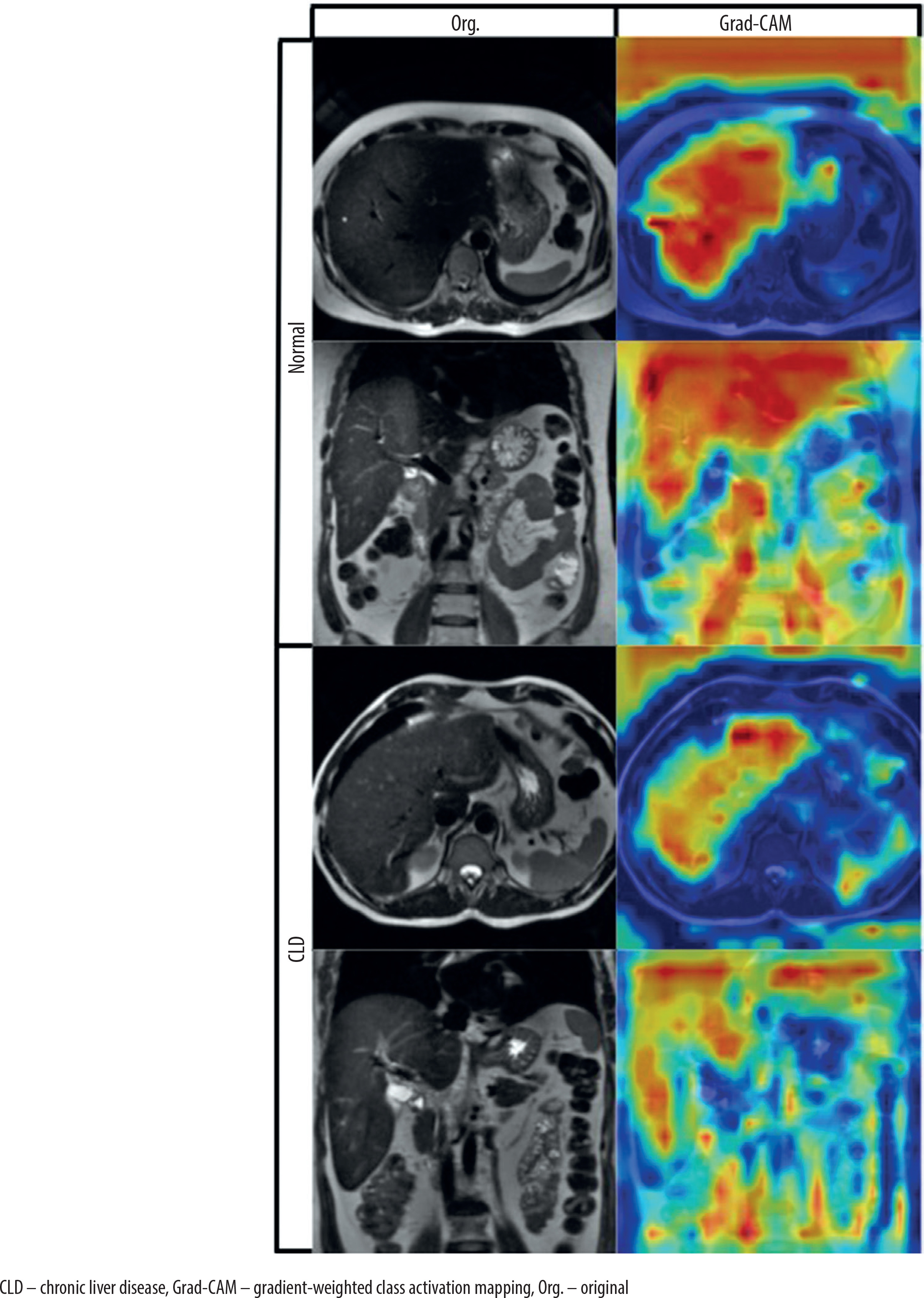
To interpret the model’s decision-making process, we applied gradient-weighted class activation mapping (Grad-CAM) to visualize the discriminative regions used by the DeepCNN model during prediction [23]. Grad-CAM is a widely used explainability technique that generates visual heatmaps highlighting the areas of an image that most influence a model’s prediction. It works by computing the gradient of the predicted class score with respect to the feature maps of a chosen convolutional layer, then weighting and combining these maps to produce a coarse localization map. In our case, Grad-CAM was applied to the final convolutional layer (Conv4), enabling us to observe where the model was focusing during classification. Representative examples of real CLD and normal cases are shown in Figure 3 to illustrate the behavior of the model.
Results
Patient data
Of the MRIs obtained from the dataset, 90 were from individuals with normal livers (45 males, 45 females) and 94 were from CLD patients (50 males, 44 females). The mean age of the patients was 53 ± 14.63 years for the entire group, 44.07 ± 12.55 years for the normal liver group, and 61.55 ± 11.06 years for the CLD group. The dataset consisted of 1112 images, of which 460 were normal liver images and 652 were chronic liver images.
Evaluation of the model
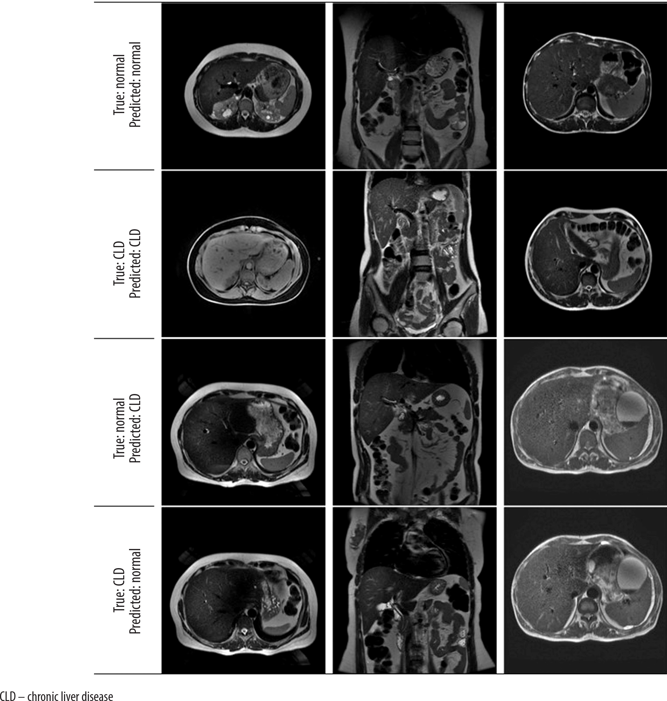
When the metrics are analyzed, according to the support criteria, there are 39 examples for class 0 (Normal) and 47 examples for class 1 (Chronic Liver). Of the model’s positive predictions for class 1 (Chronic Liver), 90.2% are considered correct, indicating a high accuracy in the model’s positive predictions. For class 1, 97.9% of the true positive samples were correctly predicted, showing that the model accurately predicted the majority of the positive class. The weighted average and macro average metrics reflect the model’s performance across both classes, and both measures show similar results, suggesting that the model provides balanced performance for both classes without bias. The model’s F1-score is 0.939, and its overall accuracy is 93%, meaning that 93% of all predictions were correctly classified (Table 1). All probabilistic outputs of the model on the test data are shown in Figure 4, and examples of patient images are provided in Figure 5.
Table 1
Classification report
| Precision | Recall | F1-score | Support | |
|---|---|---|---|---|
| 0 | 0.97 | 0.87 | 0.92 | 39 |
| 1 | 0.90 | 0.98 | 0.94 | 47 |
| Accuracy | 0.93 | 86 | ||
| Macro avg | 0.94 | 0.93 | 0.93 | 86 |
| Weighted avg | 0.93 | 0.93 | 0.93 | 86 |
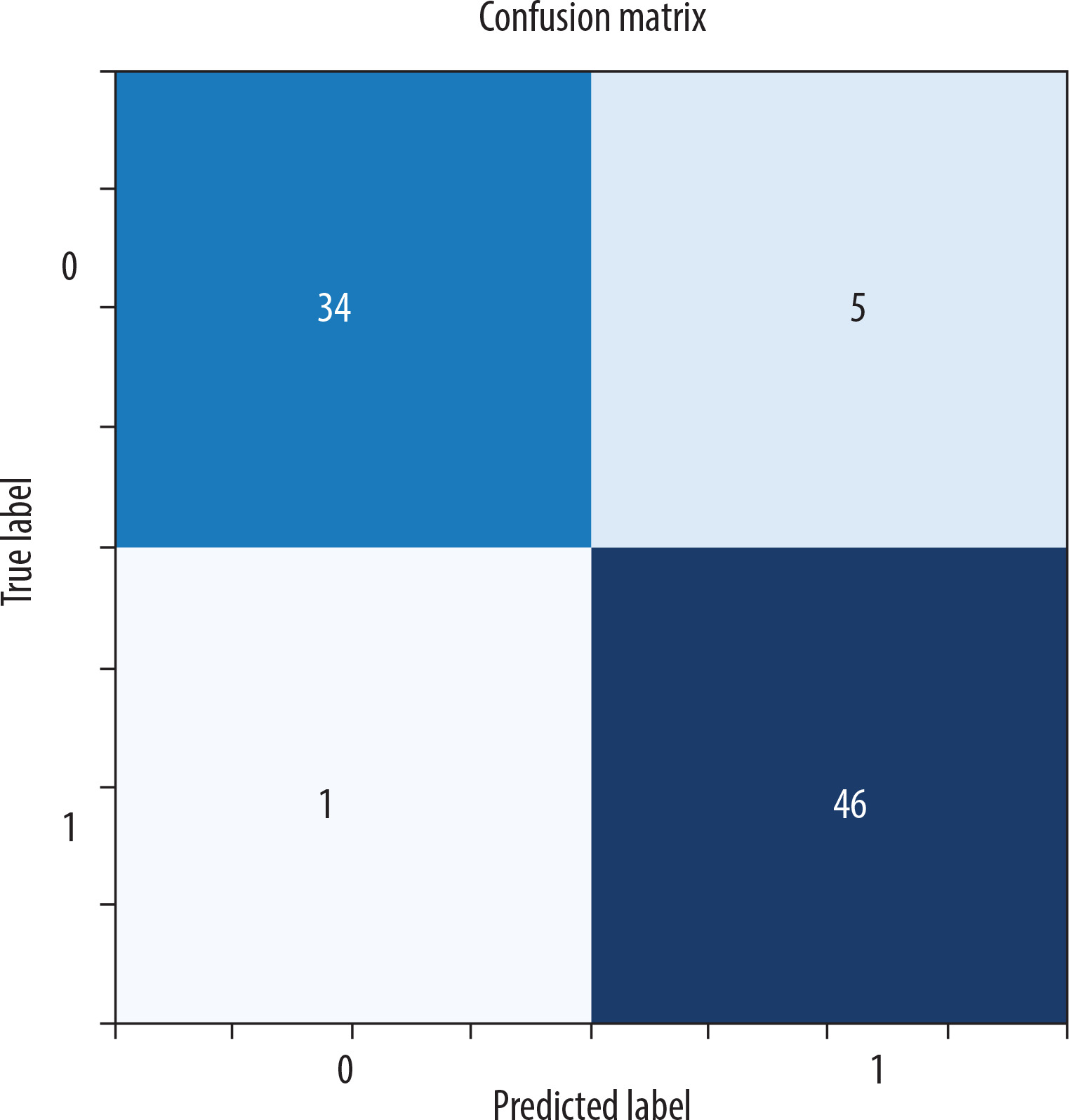
Figure 5
Axial and coronal model test prediction outputs
[The MRI dataset used in this study is not publicly available due to privacy concerns but can be requested from the corresponding author under reasonable conditions.]
A comparative experiment without data augmentation resulted in a lower test accuracy of approximately 87%, confirming that augmentation contributed positively to the model’s performance.
To better understand the model’s decision-making process, Grad-CAM visualizations are presented in Figure 3. Grad-CAM is an explainability technique that highlights the regions within an image that most influence the model’s prediction by combining the final convolutional layer’s feature maps with the corresponding gradients. Across both axial and coronal views, and for both cirrhotic and normal cases, the model was observed to focus primarily on anatomically relevant regions, particularly within or near the liver parenchyma. While minor activations outside the liver were occasionally present, these did not have a significant impact on model performance. Considering that segmentation is a time-intensive and expertise-dependent task, the ability of the model to extract meaningful features from unsegmented raw images enhances its practicality and generalizability in clinical applications.
Comparison of the model with machine learning algorithms
Logistic regression, KNN, SVM, and random forest (RF) ML methods were applied to our dataset, and the test accuracy values were obtained and are presented in Table 2.
Discussion
The model developed in our study demonstrates high precision and recall values for both classes, with a particularly notable ability to correctly identify 98% of CLD cases, indicating that the model is highly effective in detecting the disease. Although there was a slight difference in effectiveness between the two classes, this did not negatively impact the overall performance of the model. The high F1-score further confirms that the model maintains a balanced performance in terms of both precision and recall.
The model’s performance in classifying CLD and normal liver is remarkable when compared to other recent studies in the literature. The overall accuracy of this model is 93%, and the F1-score ranges between 92% and 94% across classes. This positions the model as a strong performer, particularly in complex datasets where both axial and coronal images are used together. While some other studies have reported higher accuracy rates, they generally focus on histopathological images or datasets that exclusively target liver cancer [24]. For instance, a study by Yu Sub Sung et al. [25] achieved 95% accuracy in the classification of liver diseases. However, that study focused specifically on liver cancer classification, optimizing the model for specific cancer types. In contrast, our study directly addresses CLD diagnosis and uniquely combines axial and coronal images, contributing significantly to CLD identification – a less explored area in the literature.
Additionally, a study published by Chen et al. [26] reported a 95.27% accuracy rate on histopathologic images using a Squeeze-and-Excitation Network-based DL model. This high success rate in liver cancer classification was achieved by extracting visual features through the model’s attention mechanism. However, the dataset in that study was largely limited to histopathologic images and did not incorporate data from different perspectives, such as axial or coronal images. The advantage of our model lies in its ability to integrate information from multiple imaging techniques, offering a broader application, especially in diagnosing complex diseases such as CLD. While some models in the literature achieve higher accuracy rates, this is often due to the specific type of data used or the narrow focus of the study. Our model, by contrast, stands out by effectively leveraging multiple data sources to target a specific disease.
It should also be noted that most studies in the literature utilize more limited types of data. The use of images from different viewing angles – axial and coronal planes – in this study may enhance the model’s generalizability across diverse data, though it may also increase the complexity of the learning process and, in turn, reduce performance. For this reason, many studies opt to use images from a single plane, most commonly axial. In this study, the impact of combining different planes on the learning process was also investigated [18,27].
In addition to DL models, ML models play a major role in the healthcare industry for disease prediction using various types of data from medical databases. Researchers around the world who use ML models to strategically improve medical diagnosis are achieving promising results. However, traditional ML methods have their limitations. Nilofer et al. [28] used SVM and RF methods to classify CLD, achieving approximately 85% accuracy. However, the feature engineering methods used in their study were time-consuming and error-prone, as they required manual processing of the data. Similarly, Ghosh et al. [29] employed ML algorithms such as decision tree and naive Bayes for CLD classification, but their accuracy rates remained in the 80-88% range.
In this study, ML methods were also applied to the same dataset, achieving accuracy rates ranging from 72.31% to 83.16% for different methods. This demonstrates that the DeepCNN-based model developed here provides more accurate results, aligning with findings from the literature. Compared to these results, the DeepCNN-based model’s accuracy rate of 93% shows significant progress in this field. DL has the capacity to learn more complex data structures and features, allowing for more effective feature extraction from intricate data, which in turn enables higher accuracy rates in disease diagnosis. DeepCNN networks excel at extracting the core features of the data while also discovering deeper and more meaningful patterns in the classification process.
DeepCNN outperforms traditional ML methods due to its capacity to automatically extract features and its ability to learn complex relationships in image data. This is particularly critical in diagnosing complex diseases such as CLD. The superior performance of DL methods on highly complex datasets reduces the need for manual feature engineering and yields more generalizable results.
One of the challenges in using both axial and coronal MRI data lies in their different anatomical orientations. However, our findings indicate that DL models can effectively extract meaningful patterns from both planes. The use of coronal images, although fewer in number, significantly enhanced model performance, supporting the inclusion of multi-view data in future diagnostic models.
The evaluation of the methodology presented in our study, based on the aforementioned criteria, shows that it provides an effective solution for the early diagnosis and accurate classification of CLDs, and demonstrates the applicability of DL techniques in medical image analysis. The DeepCNNs used in this study played a key role in enhancing model performance. However, there are several areas where the model can be further improved. Transformer-based models and multi-head attention mechanisms could enhance performance by enabling the model to better capture important features. Data augmentation techniques could address class imbalances and prevent overfitting. Additionally, local attention mechanisms may help the model better focus on critical regions. Finally, ensembling methods and combining different models could further improve overall performance. These improvements have the potential to increase the model’s accuracy and its effectiveness in clinical applications.
Grad-CAM analysis provided further validation for the segmentation-free approach, showing that the model was capable of attending to liver-relevant regions without requiring manual delineation. This enhances the interpretability and clinical trustworthiness of the model.
Conclusions
This study demonstrates the feasibility and effectiveness of using a DeepCNN for the classification of CLD using non-segmented MRI data. The proposed model achieved high accuracy, precision, and F1-scores, significantly outperforming traditional ML algorithms. A key contribution of this work lies in its use of raw MRI images without any manual segmentation, thereby enhancing the model’s practicality and generalizability. The automatic extraction and learning of features from raw data greatly reduce the need for manual intervention, enabling the development of more efficient and scalable diagnostic tools. This segment-free approach reduces reliance on time-consuming preprocessing steps, facilitating faster deployment in clinical settings and allowing for easier scalability across different imaging centers. Additionally, the use of different images from axial and coronal series without segmentation is crucial for the practical applicability of this DL method in clinical settings. While the results are promising, future studies should focus on multi-center validation, inclusion of clinical metadata, and the integration of advanced DL architectures such as attention mechanisms or transformer-based models. Additionally, explainable AI tools may further improve the interpretability of results, strengthening the model’s acceptability in clinical practice.In conclusion, this study contributes to the growing body of literature supporting DL in liver disease diagnosis and introduces a practical, segmentation-free approach that may serve as a foundation for more advanced, real-world AI applications in radiology.