Introduction
Tuberculosis (TB) is one of the leading causes of death worldwide. It is mainly caused by the bacterium Mycobacterium tuberculosis and affects the lungs [1]. TB spreads through the air when a person with active TB coughs, sneezes, or speaks. The common symptoms include prolonged cough, chest pain, weakness, weight loss, fever, night sweats, etc. [2]. According to the World Health Organization (WHO), delayed detection of TB can make TB more life-threatening, as well as increasing the risk of spreading the disease to others [1]. Initially, TB symptoms may be mild for many months. The main problem starts when the bacteria multiply in the body and affect different organs without being detected. Therefore, effective detection and timely treatment are crucial for full recovery and prevention of disease transmission [3].
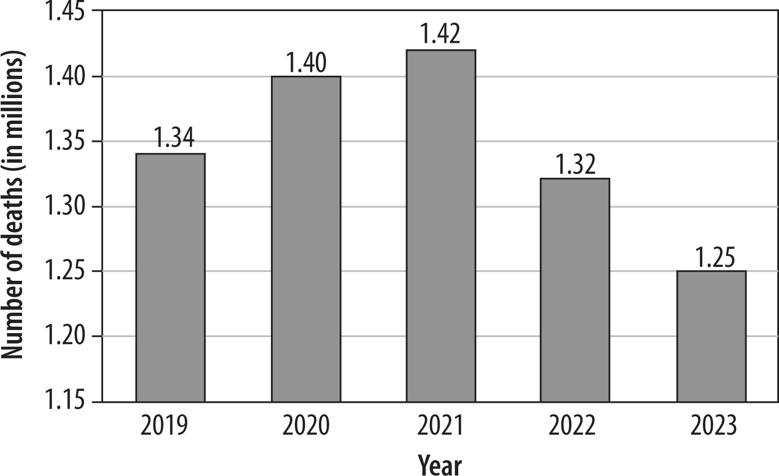
TB has become a global health issue, spreading in almost all countries and affecting all age groups. According to a WHO report, in 2023, an estimated 1.25 million people died from TB, and the total number affected was 10.8 million, including 6.0 million men, 3.6 million women, and 1.3 million children [1]. Figure 1 provides detailed statistics on the number of deaths worldwide due to TB from 2019 to 2023 [4]. Although the number of deaths has been decreasing in recent years, the range is still in the millions. Even in a developed country such as the United States of America, a total of 9,633 TB cases were reported in 2023, which is an increase of 1,295 cases from 2022 [5]. Most of those infected with TB were in the WHO regions of South-East Asia (45%), Africa (24%), and the Western Pacific (17%), with lower proportions in the Eastern Mediterranean (8.6%), the Americas (3.2%), and Europe (2.1%) [6].
There are many tools and technologies in the medical sector to detect TB. According to an international report, sputum tests are the primary method for the detection of TB in low and middle-income countries [7]. However, there are some limitations, notably the cost of sputum tests, which can vary according to the type of test and the location. Moreover, it is a time-consuming test that takes at least 24 hours to a week [7]. The other ways to detect TB are skin tests, blood tests, molecular tests, and so on. However, these are time-consuming and costly as well. Some countries do not have all of these facilities in medical centers or clinics. Fortunately, chest X-ray (CXR) images can show irregular patches in the lungs, which are typical of active TB disease [8]. This technique is also available in most countries worldwide and is cost-effective. In the manual screening of CXR images, expert and experienced radiologists or clinicians detect TB-related abnormalities (e.g., infiltrates, consolidations, cavities, calcifications, fibrosis) with close attention and care. However, this detection can be time-consuming and error-prone, particularly with subtle or atypical findings. Here, computer-aided detection and diagnosis using CXR images have shown potential for faster and more accurate assessment over the last two decades [9].
Deep learning (DL) methods such as convolutional neural networks (CNNs) are successfully used as tools for the detection and analysis of visual data, including CXR images [10]. Pre-trained CNN models – including DenseNet121, DenseNet169, DenseNet201, ResNet152, VGG19, Inception, and ResNetV2 – can be used as effective feature extractors. For prediction, machine learning (ML)-based models – such as support vector machine (SVM), XGBoost, logistic regression (LR), and DL-based custom models – can be effective classifiers. Additionally, image preprocessing techniques – such as contrast limited adaptive histogram equalization (CLAHE), Laplacian Filter, resizing, normalization, and data augmentation – can be very fruitful. The preprocessing techniques help improve the model’s accuracy.
The major contribution of this study is the effective detection of TB from CXR images using DL and ML techniques. The effectiveness is evaluated with credible evaluation metrics, curves, and graphs. Additionally, a detailed comparison of our detection performance with that of state-of-the-art related works has been provided.
The current section provides the introduction to the paper. Section II provides a literature review of the state-of-the-art related works. Section III provides a detailed explanation of the methodology for this study, explaining tools and technologies, datasets, data pre-processing techniques, etc. Section IV contains the main findings and outcomes of our study. Section V explains the study limitations and future directions. Finally, Section VI concludes and summarizes the entire study.
Related works
TB has remained a major cause of mortality globally in recent decades. The disease deserves an all-out effort in detection to ensure proper prevention and cure. In this section, we review the state-of-the-art literature on the detection of TB.
Ananya Ganapathy et al. [11] detected acute TB by combining vision language models (VLMs) using sigmoid language image pre-training for visual encoding and Gemma-3b as the transformer decoder. They considered CXR images (100,000 TB-annotated) and clinical notes (symptoms and risk factors) to build a multimodal framework. For preprocessing, they applied image patching (16 × 16) on 224 × 224 resolution X-ray images, token embeddings, and masked modeling techniques (masked image modeling and masked language modeling). Their VLM-based model achieved the highest performance in detecting nodules.
Nagireddy Maheswari et al. [12] detected TB by following Preferred Reporting Items for Systematic Reviews and Meta-Analyses (PRISMA) guidelines with SVM, Random Forest, LR, InceptionV3, and MobileNet models. They considered CXR images from standard datasets, including the Shenzhen dataset, and used CLAHE and equalizeHist as image preprocessing techniques. They obtained the highest performance with the SVM model.
Vo Trong Quang Huy et al. [13] developed an improved DenseNet, a Deep Neural Network model for TB detection using CXR images from standard datasets, including the Shenzhen dataset. A new DL model was proposed to detect TB with CXR images. The model is based on the convolutional block attention module (CBAM) and the wide dense net (WDnet) architecture, which is designed to capture spatial and contextual information in the images effectively. The performance of the developed model (named CBAMWDnet) was evaluated based on a large dataset of the CXR images, and it was found to outperform other models considered.
Eman Showkatian et al. [14] proposed DL-based automatic detection of TB. They considered two publicly available standard datasets, including the Shenzhen dataset. Pre-trained CNN models, such as InceptionV3, Xception, ResNet50, VGG19, and VGG16, were used to classify TB and healthy control cases from the CXR images. A custom CNN yielded a moderate outcome, whereas Xception, ResNet50, and VGG16 achieved the best results.
Mohammad Alsaffar et al. [15] detected TB from CXR images using three different classification methods: SVM, LR, and nearest neighbors. Features were extracted using a CNN model, ResNet50.
Tawsifur Rahman et al. [16] used a total of 9 pre-trained deep CNN models to classify TB and non-TB CXR images. Additionally, U-net models were employed. They considered the National Library of Medicine dataset, the Belarus dataset, the NIAID TB Portal Program dataset, and the RSNA Pneumonia Detection Challenge dataset.
Tae Hoon Kim et al. [17] proposed the tuberculosis semantic segmentation-guided CNN (TSSG-CNN) model, which combines semantic segmentation and an adaptive CNN architecture for enhanced detection of TB. The study considered a dataset consisting of 566 CXR images from Shenzhen Hospital (the Shenzhen dataset), manually annotated with lung masks. The training, validation, and test ratios were 12, 5, and 1 batch, respectively. The TSSG-CNN model outperformed other models, including simple CNNs, batch normalized CNNs, and dense CNNs.
Reshma SR et al. [18] demonstrated that contour extraction, ellipse detection, and ellipse merging techniques could be used to count M. tuberculosis bacteria on 176 CXR images from 10 countries across Africa, Asia, and Europe. They used data augmentation and attention pooling as preprocessing techniques. The limitations of their work are the domain shift and dataset size constraints.
Joong Lee et al. [19] identified the Neural Architecture Search (NAS) Network as the best-performing model (NASNet-A Large) in TB detection from histopathological lung tissue images. They implemented other DL feature extractors such as ResNet50, Inception v3, Xception, DenseNet169, EfficientNet-B0, RegNetY-064, Vit_base_patch16_224, and Swin Transformer Small. They used autopsy specimen datasets to conduct the study. A limitation of their study is the use of a single imaging modality.
Wong et al. [20] introduced a self-attention Deep CNN model, named TB-Net, designed for TB detection. They considered a multinational patient dataset of 6,939 (positive: 3,461, negative: 3,478) chest radiographs. The dataset was compiled using data from various organizations, repositories, and datasets, including the Shenzhen dataset. They achieved an outstanding performance with TB-Net.
Dasanayaka and Dissanayake [21] proposed a DL architecture for TB diagnosis using a total of 2,770 (positive: 1,393, negative: 1,377) CXR images from standard datasets, including the Shenzhen dataset. Their model achieved significant accuracy. The model’s performance is also reflected in its Youden’s index of 0.941, which represents excellent diagnostic capability in distinguishing TB-positive cases from healthy controls.
Singh et al. [22] detected TB using CXR images from Indian datasets, which contain over 1,000 CXR images, labeled as healthy control and TB-positive samples. The authors experimented with pre-trained deep CNN models such as AlexNet, GoogLeNet, and ResNet. The preprocessing involved image resizing, histogram equalization, and image normalization. The limitations of the study include a class imbalance issue that influenced overall model performance.
Material and methods
Methodology
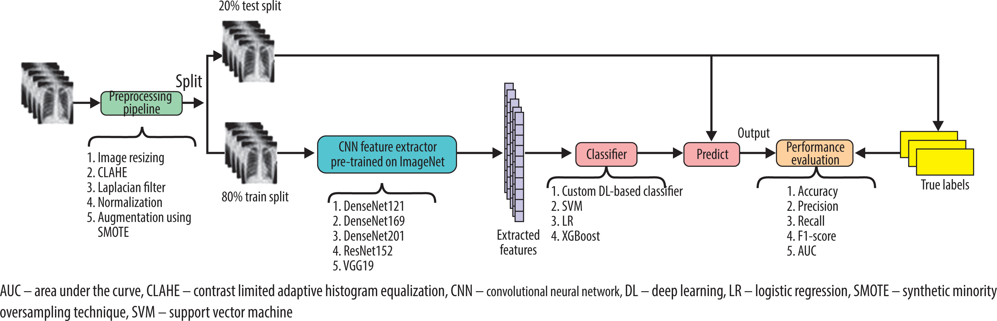
The architecture of the proposed approach is illustrated in Figure 2, which presents a schematic overview of the entire methodology. It provides a detailed description of the analysis and classification of CXR images through a series of interrelated steps. We used DL-based CNN feature extractor models such as DenseNet121, DenseNet169, DenseNet201, ResNet152, and VGG19. The models are pre-trained on the ImageNet dataset. In a determining role, we used a DL-based classifier. Additionally, ML models such as SVM, XGBoost, and LR are used as classifiers, which automate the diagnostic process. The basic idea is to remove the top classification layer of the feature extractor models and add the ML-based and DL-based custom classifiers for classification. In Algorithm 1, we present the procedure for the DL-based custom classifier. We have provided appropriate comments in the algorithm to explain each of the steps clearly. For the classifiers, significant hyperparameters such as learning rate, batch size, number of epochs, optimizer, loss function, dropout rate, etc., have been optimized for achieving the best detection performance possible. The output of this study has been evaluated by some credible performance evaluation metrics, such as accuracy (1), precision (2), recall (3), F1-score (4), and AUC.
Algorithm 1: AddFinalClassifierHead
Input: Feature Extractor model FEmodel
Output: FEmodel with a Binary Classifier,
FEmodel ← GlobalAveragePooling2D(FEmodel)
# Reduce spatial dimensions by computing the global average
FEmodel ← DenseLayer (units = d1_layers, activation = ReLU, L2_regularization = 0.001)(FEmodel)
# 1st fully connected layer with d1_layers, ReLU activation, and L2 regularization
FEmodel ← BatchNormalization(FEmodel)
# Normalize activations to stabilize and accelerate training
FEmodel ← Dropout(do1_rate)(FEmodel)
# Apply dropout (1st) to reduce overfitting with dropout rate, do1_rate
FEmodel ← DenseLayer(units = d2_layers, activation = ReLU, L2_regularization = 0.001)(FEmodel)
# 2nd fully connected layer with d2_layers, ReLU activation, and L2 regularization
FEmodel ← Dropout(do2_rate)(FEmodel)
# Apply dropout(2nd) with dropout rate, do2_rate
FEmodel ← DenseLayer(bc_layers = 1, activation = Sigmoid) (FEmodel)
# Final binary classification layer and sigmoid activation
ReturnFEmodel
ReLU – rectified linear unit
To visualize the detection performances, the following graphs and curves are presented: confusion matrix (CM), recall versus precision curve, receiver operating characteristic (ROC) curve, training versus validation accuracy and loss, loss versus learning rate curve, precision, recall, and F1-score versus epochs curve.
Datasets description and preparation
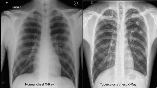
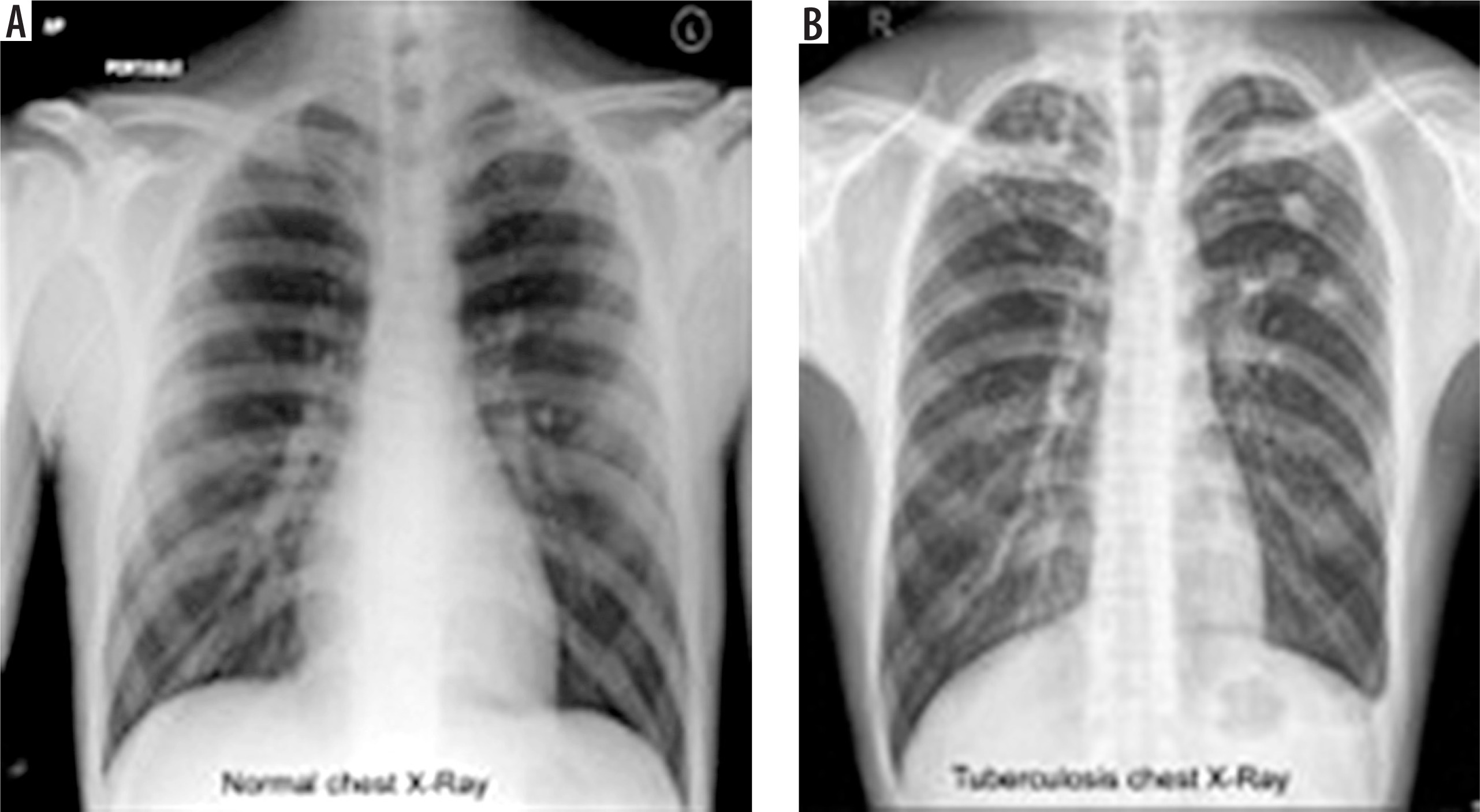
In this study, we used CXR images to detect TB. In Figure 3, CXRs of a healthy (healthy control case) person and a TB patient are depicted for visualization and comparison.
The three datasets used in our study are the TB CXR database [23], the TB CXR or Shenzhen dataset [24], and CXR TB from India [25].
The first dataset was created by researchers from Bangladesh and Malaysia. From this dataset, we considered a total of 1,574 CXR images, including 847 healthy control and 700 TB-infected images. From the second dataset, we considered 326 healthy control and 336 TB-infected CXR images, making a total of 662 CXR images. For the last dataset, we considered a total of 155 CXR images, including 77 healthy control and 78 TB-infected CXR images. Finally, our dataset consisted of 2,391 CXR images, including 1,277 healthy control and 1,114 TB-infected CXR images. Table 1 summarizes the datasets.
Table 1
Summary of chest X-ray (CXR) datasets for tuberculosis (TB) detection
| Datasets | Healthy control CXR | TB-infected CXR | Total images |
|---|---|---|---|
| TB CXR database | 874 | 700 | 1574 |
| TB CXR (Shenzhen) | 326 | 336 | 662 |
| TB CXR from India | 77 | 78 | 155 |
| Entire dataset | 1277 | 1114 | 2391 |
The dataset was divided into two parts, where 80% was taken for training the model to learn and detect the patterns, and the remaining 20% was left for testing to observe the classification performance. We used the synthetic minority oversampling technique for the CXR imageaugmentation to improve the generalization of different models [26]. To improve image analysis, we used some robust preprocessing techniques such as CLAHE [27] (for enhancing contrast in CXR images), Laplacian Filter [28] (for sharpening images to highlight details), image resizing (for ensuring a fixed input size), and normalization (for scaling values for better model performance).
Experimental setup
We used Python as the scripting language to implement our methodology. As a framework, TensorFlow/Keras was used in the Kaggle platform [29]. Memory (RAM), computation power of GPUs and CPUs, etc., were used from the Kaggle platform.
Results and discussion
Detailed explanation of results
Table 2 presents the detailed outcomes of this study. We evaluated a total of 20 combinations of feature extractors and classifier models, where we implemented each feature extractor with all the considered classifiers. Each model’s outcomes are described under accuracy, precision, recall, F1-score, and AUC. In evaluation, we considered class-wise detection performance for precision, recall, and F1-score. In Table 2, class 0 resembles the class with healthy images, and class 1 resembles the class with TB-infected CXR images. Additionally, we provided the macro average (Mac Avg.) and weighted average (Wtd. Avg.) of the class performances. We found that ResNet152, DenseNet169, and DenseNet201 were the best-performing feature extractors, whereas the SVM classifier and the DL-based custom classifier were found to be the best classifiers. ResNet152 with an SVM classifier achieved the highest accuracy of 99.91%. DenseNet169 and the custom DL-based classifier achieved the highest precision, recall, and F1-score of 99.22%, 99.23%, and 99.22%, respectively, considering both the Wtd. Avg. and Mac Avg. Lastly, DenseNet201 and the custom DL-based classifier achieved the highest recall, F1-score, and AUC of 99.99%, considering both the macro and weighted averages. After observing the overall performances, we propose DenseNet169 and the custom classifier as the best performers due to their high and well-balanced values in evaluation metrics. The highest performances as well as the highest performer are marked in bold in Table 2. In Table 3, the fine-tuned or optimized hyperparameters are presented.
Table 2
Performance comparison of various classifiers using different pre-trained feature extractors
Table 3
Optimized hyperparameters for various classifiers
State-of-the-art comparison
Table 4 compares our detection performance to that of state-of-the-art studies. The asterisk-marked related works and this work share the same Shenzhen dataset. Additionally, the proposed model of this study is highlighted in bold. Moreover, the underlined values are the best achieved performances among the related works.
Table 4
Performance comparison of tuberculosis detection models
| Models | Accuracy (%) | Recall (%) | Precision (%) | F1-score (%) | AUC (%) |
|---|---|---|---|---|---|
| VLM [11] | – | 96.00 | 97.00 | – | – |
| SVM [12]* | 97.00 | 97.00 | 97.00 | 97.00 | – |
| DNN [13]* | – | 98.80 | 94.28 | 96.35 | – |
| VGG16 [14]* | 90.00 | 91.00 | 91.00 | 91.00 | 91.00 |
| ResNet50+SVM [15] | 87.00 | 87.00 | 88.00 | 87.00 | – |
| U-Net + DenseNet201 [16] | 98.60 | 98.56 | 98.57 | – | – |
| TSSG-CNN [17]* | 98.75 | – | – | 98.70 | – |
| TB-Net [20]* | 99.86 | 100.0 | – | – | – |
| Ensemble model (VGG16 + inceptionV3) [21]* | 97.10 | 97.90 | – | – | – |
| ResNet101 [22] | 93.40 | 92.90 | – | – | – |
| ResNet152 + SVM Classifier | 99.91 | 99.02 | 99.02 | 99.02 | 99.91 |
| DenseNet169 + custom classifier (proposed) | 99.22 | 99.22 | 99.23 | 99.22 | 99.91 |
| DenseNet201 + custom classifier | 99.22 | 99.22 | 99.22 | 99.22 | 99.99 |
We found that the TB-Net model [20] achieved the highest accuracy of 99.86% and the highest recall of 100.0% among the related works, while the U-Net + DenseNet201 [16] model achieved the highest precision of 98.57%. The TSSG-CNN [17] model achieved the highest F1-score of 98.70%. Lastly, the VGG16 [14] model achieved the highest model AUC of 91.00%. The highest achieved detection performances of this work are provided in the last three rows of Table 4. We can observe that our study has achieved the highest in almost all the evaluation metrics, including accuracy of 99.91% (ResNet152 + SVM Classifier), precision of 99.23% (DenseNet169 + Custom Classifier), an F1-score of 99.22% (DenseNet169 + Custom Classifier), and AUC of 99.99% (DenseNet201 + Custom Classifier). In this comparison, the values of both macro and weighted averages for recall, precision, and F1-score are applicable as they provide the same result. However, we failed to achieve a higher recall than the recent works.
Graphs and charts
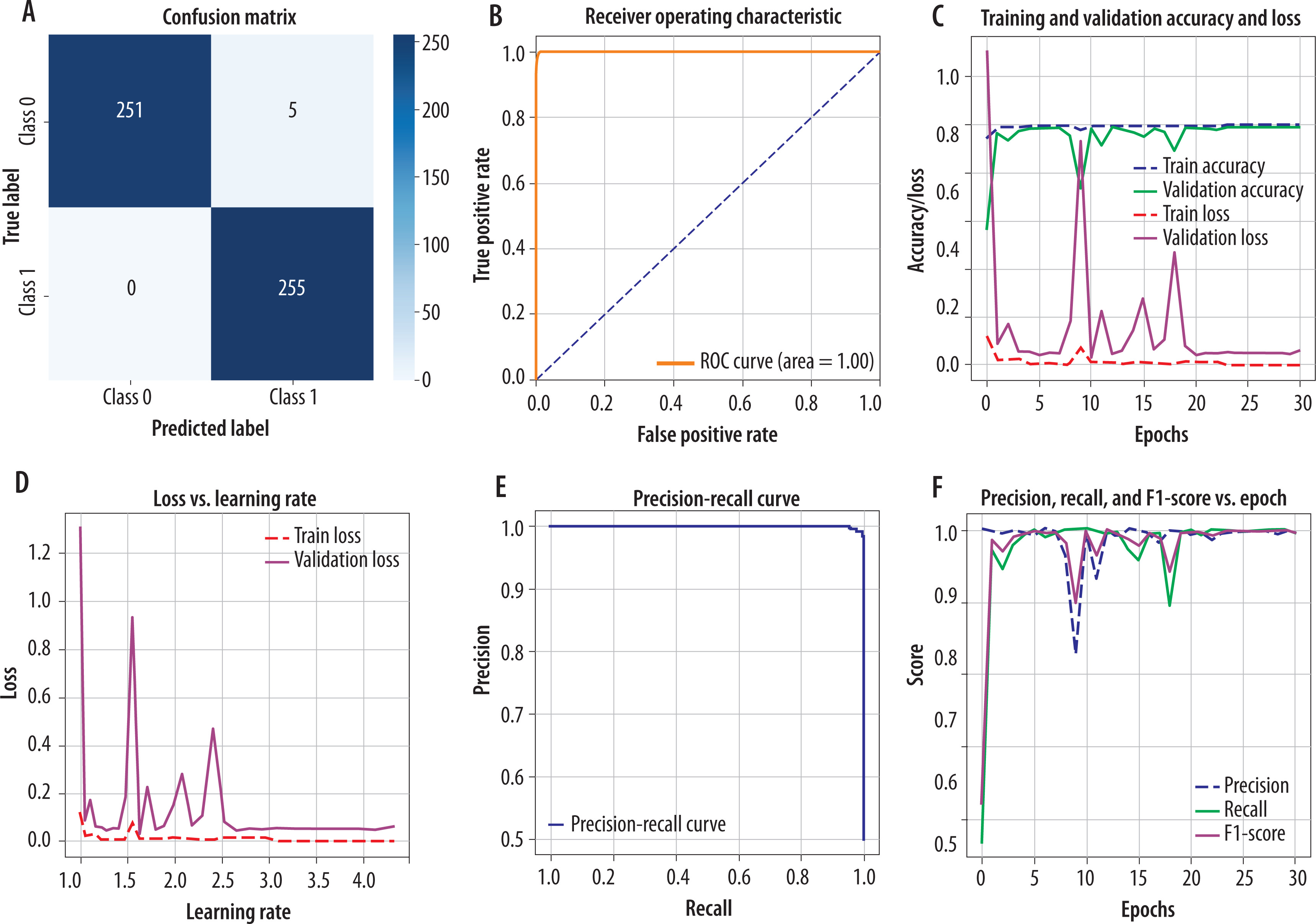
Figure 4 presents CM and other related curves and graphs of our proposed model, DenseNet169 with the custom classifier. Figure 4A is a CM that illustrates high true positive rates and high true negative rates, exhibiting excellent classification performance, as there are very few misclassifications. Figure 4B represents the ROC AUC curve where the curve is close to the top left corner, representing a better model. Here, AUC is 1.00, indicating perfect model discrimination between TB-infected and healthy control cases. Figure 4C is a graph of training and validation accuracy and loss, which shows how the model improves in accuracy with a decrease in loss after each epoch. Generally, the validation accuracy should increase while the loss should decrease. Although there are a few spikes in the curve, they are negligible. Figure 4D presents a graph of loss versus learning rate, providing information about the change in loss when the model is trained under different learning rates. Despite having some spikes, it exhibits good condition. Figure 4E is a graph of the precision versus recall curve, exhibiting a trade-off between precision and recall. The curve is close to the top-right corner, indicating high precision and recall, which reflects a well-performing model, especially valuable for imbalanced datasets. Figure 4F is a graph of precision, recall, and F1-score versus epochs, which represents the changes in precision, recall, and F1-score with epochs. Here, the metrics remained consistently high across epochs, validating the model’s robustness and stability during training.
Discussion
Our proposed methodology has achieved a significant performance compared to that of the state-of-the-art studies, as discussed in the previous subsections. The evaluated DL and ML models for feature extraction and classification also performed well. The selected image pre-processing techniques have proven to be robust. Additionally, the hyperparameters are optimized effectively to yield an acceptable performance. The performance metrics, graphs, and curves effectively demonstrate the achieved performances.
Limitations and future work
There are a few limitations of this study that offer opportunities for future improvement. Firstly, we failed to achieve a higher recall with our evaluated models than that of the existing works. Secondly, although we considered a sufficiently large and well-balanced dataset within available resource constraints, a larger dataset could be constructed with more datasets, repositories, or sources. This would increase the dataset size, generality, and diversity, which might better reflect real-world variations. Finally, the methodology of this study can be enhanced by considering hybrid as well as ensemble learning models.
Conclusions
TB is a serious global health issue. In 2023, TB-infected cases numbered 10.8 million, and of these, 1.25 million people died. Therefore, the global risk of TB remains high. However, standard TB testing is labor-intensive, time-consuming, and costly. In response to this challenge, there can be effective attempts to develop an automated TB detection system deploying DL and ML approaches with CXR images. In this study, we evaluated the performance of five DL CNN-based feature extractors pre-trained on the ImageNet dataset and a DL-based custom classifier in TB detection. Additionally, ML-based classifiers were considered. A total of 3 datasets of CXR images were used. ResNet152, DenseNet169, DenseNet201, SVM, and DL-based custom classifiers emerged as the best performersin various evaluation metrics. Among the well-performing models, we propose DenseNet169 with a custom classifier as the best one due to its achievement of high and well-balanced performance (accuracy: 99.22%, precision: 99.23%, recall: 99.23%, F1-score: 99.22%, and AUC: 99.98%). This study contributes to advancing the automated detection of TB, providing more reliable support to physicians. In future research, we aim to enhance the overall performance of our methodology by expanding the data domain and integrating more robust detection strategies.